
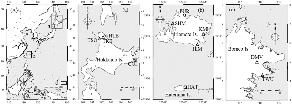
Fig. 1.
Location of the observation sites. (a) Hokkaido Island, which is located in the northern part of Japan. (b) Iriomote Island and Hateruma Island, which are located in the southeastern part of Japan. (c) Sabah, Malaysia, which is located in the northeastern part of Borneo Island. Circles are the observation sites for continuous CO2 measurements. Triangles are the observation sites for CO2 sonde and continuous CO2 measurements. Squares are the reference (background) sites used for the circles and triangles. (d) Borneo’s reference (background) site is located around 5°N, 150°E in the Pacific Ocean (shipboard measurements) (close up image not shown).
Table 1.
Summary of the observation sites used in this study.
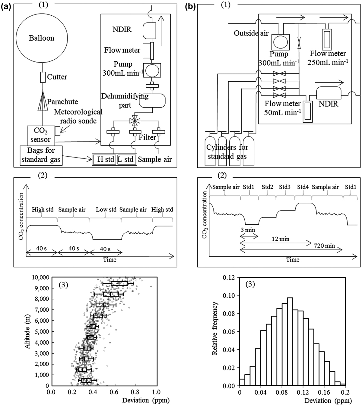
Fig. 2.
(a) These images show the (1) schematic, (2) measurement sequence and (3) standard (for 40 s) deviation as a function of altitude for the CO2 standard gases measured with the CO2 sonde. The standard deviation of the CO2 sonde data was calculated from the analysed values for both high and low standard gases over 40 s. A total of 18 CO2 sonde measurements were used for the calculations (at Hokkaido, Iriomote and Borneo, where the sonde was launched on September 2012, September 2013 and August 2015, respectively). (b) These images show the (1) schematic, (2) measurement sequence and (3) relative frequency of the standard deviation for CO2 standard gases measured with continuous CO2 measurements. The standard deviation of the continuous CO2 measurement data was calculated from the analysed values for each of four standard gases over 3 min. The observational results at Hokkaido (from August 2012 to September 2013), Iriomote (from July 2013 to December 2015) and Borneo (from January to December 2015) were used for the calculations.
Table 2.
Location and time of the CO2 sonde and continuous measurements.
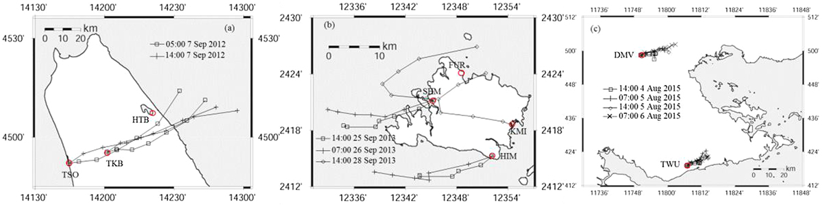
Fig. 3.
Flight paths every 10 min for the horizontal direction of CO2 sonde measurements taken in (a) Hokkaido, (b) Iriomote and (c) Borneo. The CO2 sonde was launched twice at Hokkaido, three times at Iriomote, and four times at Borneo. The CO2 sonde rises at about 1200–1800 m per 10 min.
Table 3.
The height of the stable boundary layer (SBL) and convective planetary boundary layer (CBL) and average CO2 concentrations inside the SBL and CBL.
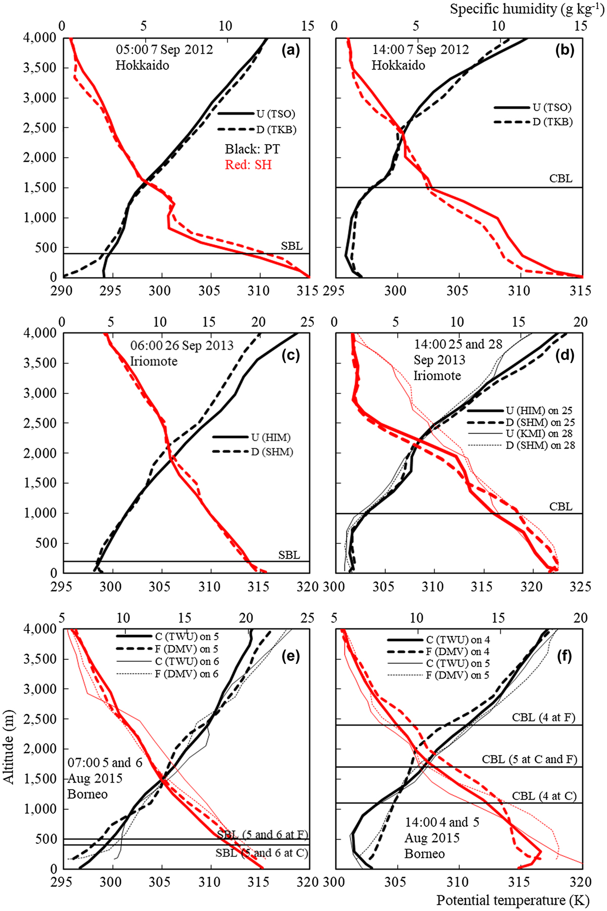
Fig. 4.
Vertical profiles of potential temperature and specific humidity at (a) 05:00 on 7 September 2012 in Hokkaido, (b) 14:00 on 7 September 2012 in Hokkaido, (c) 06:00 on 26 September 2013 in Iriomote, (d) 14:00 on 25 and 28 September 2013 in Iriomote, (e) 07:00 on 5 and 6 August 2015 in Borneo, and (f) 14:00 on 4 and 5 August 2015 in Borneo. Black lines are the potential temperature, and red lines are the specific humidity. Solid lines show the upwind sites (Hokkaido and Iriomote) and coast site (Borneo), and dashed lines show the downwind sites (Hokkaido and Iriomote) and forest site (Borneo). The height of the stable boundary layer (SBL) and planetary boundary layer (PBL) are also shown (see text).
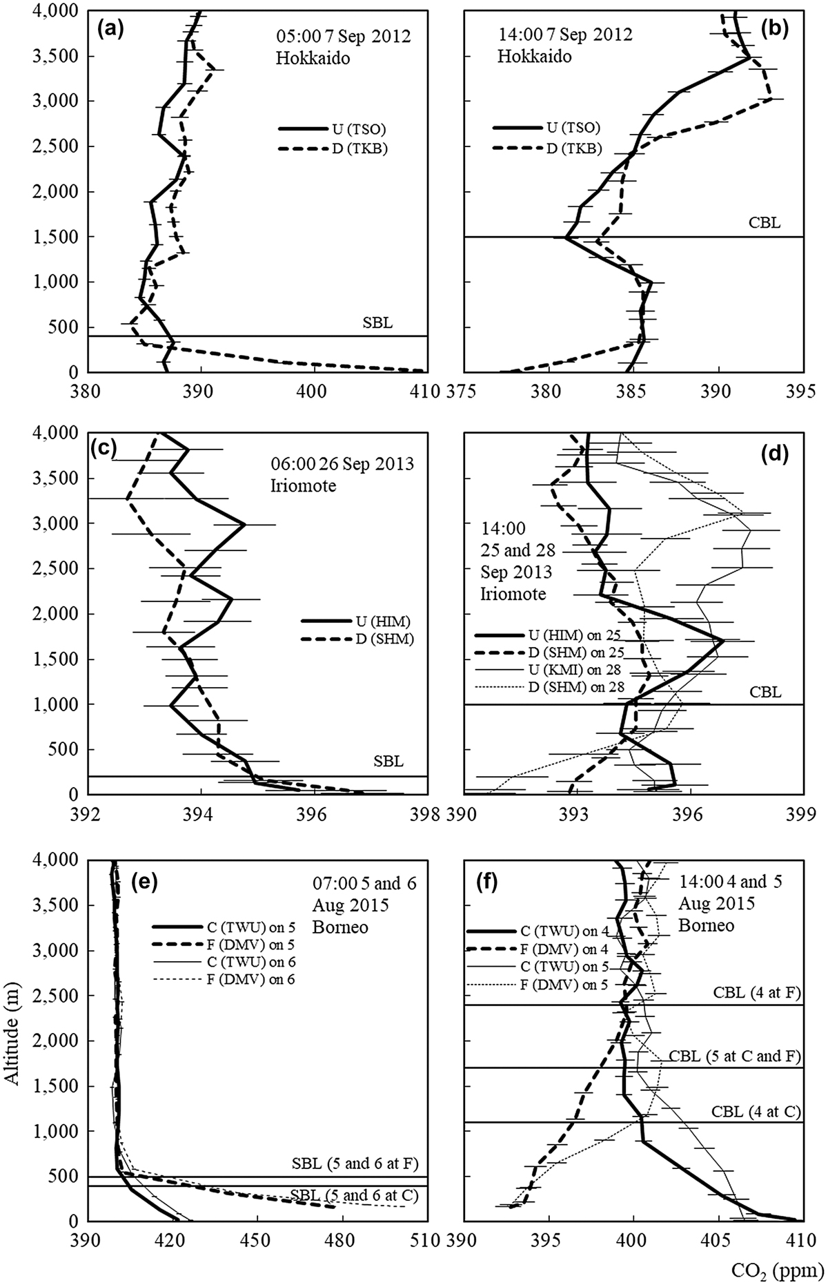
Fig. 5.
Vertical profiles of atmospheric CO2 concentrations at (a) 05:00 on 7 September 2012 in Hokkaido, (b) 14:00 on 7 September 2012 in Hokkaido, (c) 06:00 on 26 September 2013 in Iriomote, (d) 14:00 on 25 and 28 September 2013 in Iriomote, (e) 07:00 on 5 and 6 August 2015 in Borneo, and (f) 14:00 on 4 and 5 August 2015 in Borneo. Solid lines show the upwind sites (Hokkaido and Iriomote) and coast site (Borneo), and dashed lines show the downwind sites (Hokkaido and Iriomote) and forest site (Borneo).
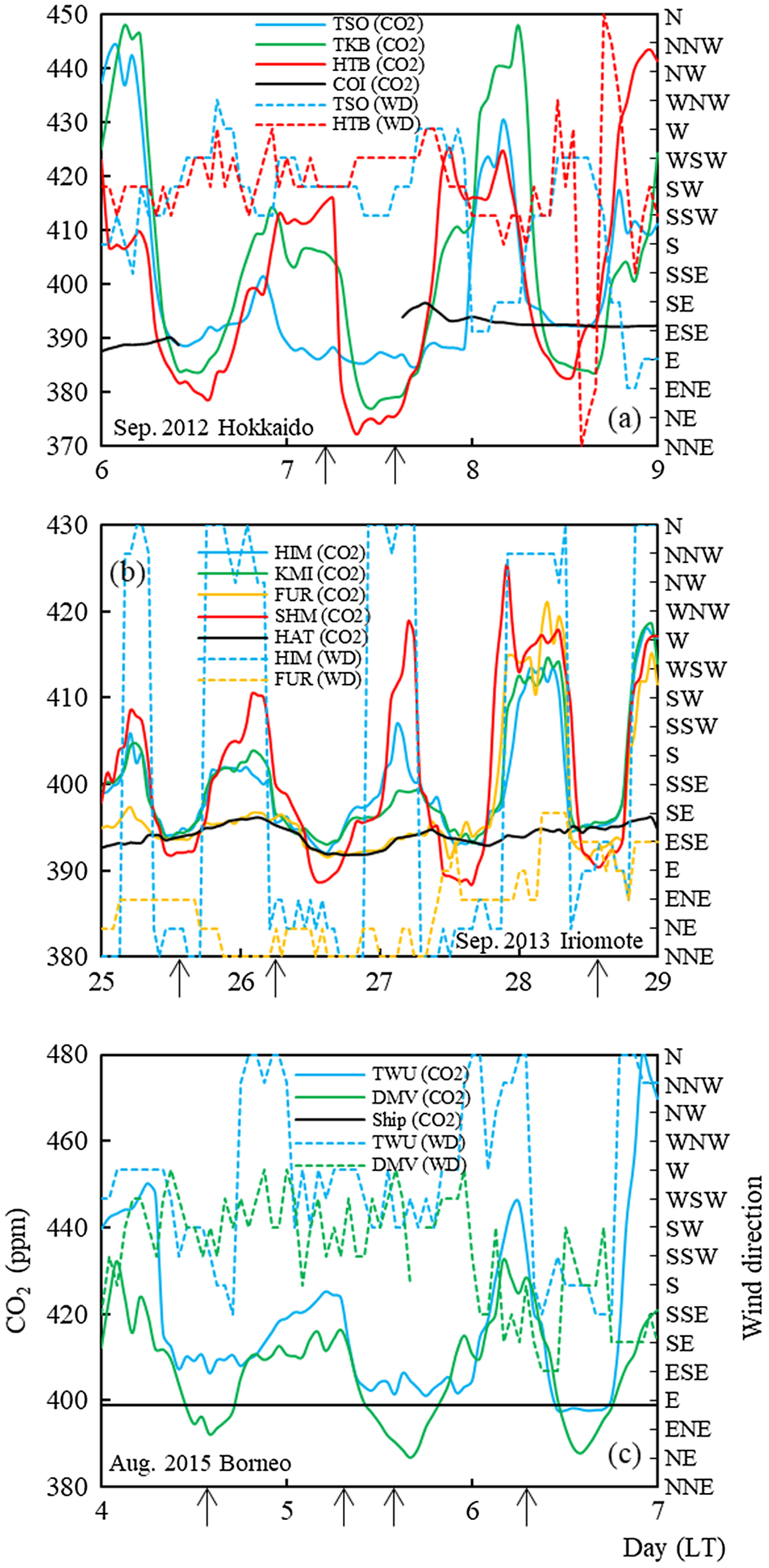
Fig. 6.
Diurnal variations of CO2 concentrations (solid lines) and wind direction (dashed lines) near the ground in (a) Hokkaido on 6–8 September 2012, (b) Iriomote on 25–28 September 2013 and (c) Borneo on 4–6 August 2015. The black lines show the background CO2 concentrations obtained from (a) Cape Ochiishi on 6–8 September 2012, (b) Hateruma Island on 25–28 September 2013 and (c) shipboard measurements taken on 19 August 2015 at 5°N, 148°E. Arrows indicate the time for the launch of the CO2 sonde.
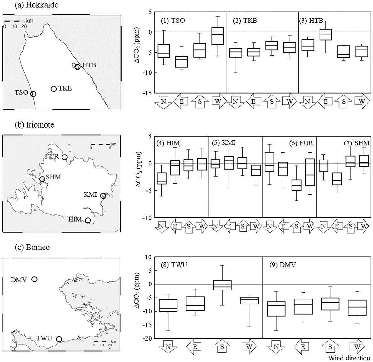
Fig. 7.
Differences in CO2 concentration from the background level at 2 pm (ΔCO2) as a function of wind direction at (1) TSO, (2) TKB, (3) HTB, (4) HIM, (5) KMI, (6) FUR, (7) SHM, (8) TWU and (9) DMV. The median value (the line in the box), inner 50th percentile of the value (box), and inner 95th percentile of the value (bars) for the ΔCO2 are shown. The observational data used here were collected from August to September 2012 and from July to September 2013 in Hokkaido, from July to September 2013, 2014 and 2015 in Iriomote, and from July to September 2015 in Borneo, and we used all of the data from the above observation periods when we produced Fig. 8. For the wind direction analysis, north includes NW–N–NE, east includes NE–E–SE, south includes SE–S–SW and west includes SW–W–NW.
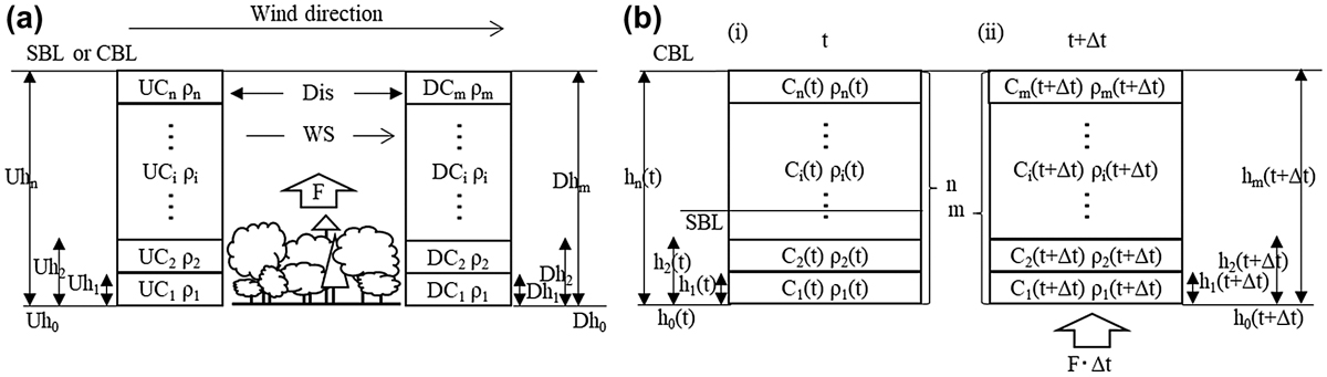
Fig. 8.
Box model for the estimation of the CO2 flux in (a) Hokkaido and Iriomote and (b) Borneo. (a) F is the CO2 flux (μmol m−2 s−1); UC i and DC i are the CO2 concentrations (ppm) in the i-th layer of the vertical profiles at the U (upwind site) and D (downwind site), respectively; Uh n and Dh m corresponds to the CBL height (m) at the U and D sites (Table 3) (usually they are set equal); ρ i is the molar air density (mol m−3); WS is the average wind speed of layers under CBL (m s−1) obtained from the flight path of the sonde; and Dis is the distance between the upwind site (or coast) and downwind site (m). (b) F is the CO2 flux (μmol m−2 s−1); C i (t) and C i (t + ∆t) are the CO2 concentration (ppm); h i (t) and h i (t + ∆t) are the height (m) of the i-th layer at the moment of t and t + ∆t, respectively; h n (t) is the same as h m (t + ∆t), corresponding to the CBL height (m) (Table 3); ρ i (t) and ρ i (t + ∆t) are the molar air density (mol m−3); and ∆t is 7 h or 17 h.
Table 4.
Estimated CO2 flux in the three forests.
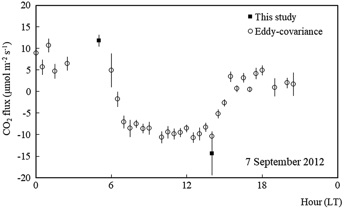
Fig. 9.
CO2 flux estimated by this study and by the eddy-covariance method in Hokkaido on 7 September 2012. This study’s values were calculated from the differences in CO2 concentrations between the upwind site and downwind site. The values from the eddy-covariance method were observed at the Teshio Experimental Forest of Hokkaido University near the TKB site (Takagi et al., 2009). Error bars of the eddy-covariance in the figure show the random sampling error in each flux as determined in accordance with Finkelstein and Sims (2001).
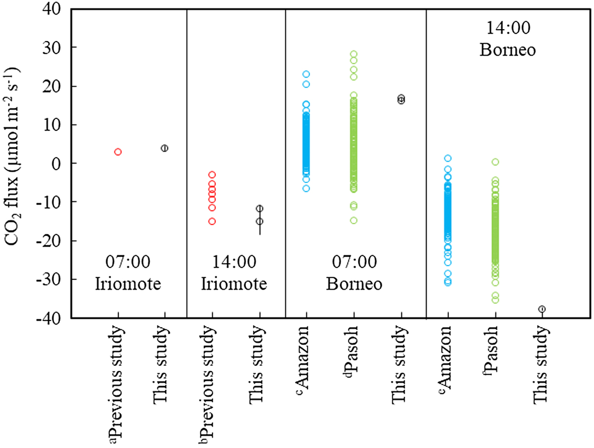
Fig. 10.
Comparison of the estimated CO2 fluxes obtained in this study and in previous studies.
aCO2 flux at Iriomote from noon to 17:00 in March and November 1991 and July 1992 (Yamamoto et al., 1996). bSame as a but from 05:00 to 07:00 in July 1992. cHourly CO2 flux at 05:00 in the Santarem-km67-Primary Forest, Amazon (latitude: 2°51′24.1″S, longitude: 54°57′32.0″W), in August from 2002 to 2011 (though data for 2006 and 2007 are not included) (Ameriflux, http://ameriflux.lbl.gov/data/download-data/). dHourly CO2 flux at 06:00 on the Pasoh Forest Reserve, Malay Peninsula (latitude: 2°58′14.6″N, longitude: 102°17′57.8″E), in August from 2003 to 2009 (Asiaflux, https://db.cger.nies.go.jp/asiafluxdb/?page_id=16). eSame as c but for noon. fSame as d but for noon.