Evaluation of forest CO2 fluxes from sonde measurements in three different climatological areas including Borneo, Malaysia, and Iriomote and Hokkaido, Japan

Introduction

1.

The estimate of the uptake of atmospheric CO₂ by the terrestrial biosphere (2.6 ± 1.2 PgC yr⁻¹ in terms of the global annual average from 2000 to 2009) (IPCC, 2013) is associated with a relatively large uncertainty compared to that by the ocean (2.3 ± 0.7 PgC yr⁻¹), and this uncertainty is partly due to the difficulties associated with estimating the variation of the land flux. Variations in the land flux are driven by the effects of disturbances and changes induced by natural and anthropogenic origins, such as changes in temperature and precipitation (Malhi and Wright, 2004), forest fires, logging practices and plantings (Amiro et al., 2006; Ramankutty et al., 2007; Hirata et al., 2014); these changes cannot easily be monitored at different temporal and spatial scales because of the complicated features of terrestrial surfaces. Nevertheless, the CO₂ flux of the terrestrial surface has to be accurately evaluated because both increases and decreases in the flux directly affect the accumulation rate of atmospheric CO₂, which is the largest driving factor for climate change. Especially in Southeast Asia, tropical forests are very important in terms of emissions from frequent large forest fire events and continuous land use change.

Methods for observing CO₂ fluxes from forests can be roughly categorized into two types of methods. One method involves the installation of a tower in a forest to measure the change of atmospheric CO₂ concentrations near the forest canopy using the eddy-covariance method at the top of the tower (e.g. Saigusa et al., 2008). This method is called the bottom-up method, and it has been carried out at many forest sites around the world. However, strictly speaking, the CO₂ flux evaluated by the bottom-up method is a very local flux, and the results are therefore limited to the forest near the tower. Hence, many tower sites are necessary to assess the CO₂ flux at the regional scale. Additionally, note that, especially in the case of tropical regions, CO₂ flux observations at night by the eddy-covariance method are difficult to undertake because of the low wind speed. Therefore, an assessment of the CO₂ flux by methods other than the eddy-covariance method is necessary. The other method involves the use of atmospheric CO₂ concentration observations and inverse-model calculations (e.g. Gurney et al., 2004; Peylin et al., 2013). This method is called the top-down method, and it actively uses global observations of CO₂ concentrations collected by satellites (e.g. the Greenhouse Gases Observing Satellite, GOSAT) in addition to background ground data in recent years (e.g. Maksyutov et al., 2013; Kondo et al., 2015). In general, inverse modelling calculations are applied to global flux evaluations at the continental scale. Therefore, when we evaluate the CO₂ flux of a regional forest for one country using the top-down method, it can be difficult to obtain accurate data because CO₂ observations by satellites and background base stations are not available at high temporal and spatial resolutions at present. In addition, the success rates for satellite observations will be limited if the targeted region is a tropical rain forest because tropical regions are typically covered by clouds, which prevent infrared (IR) absorption measurements for the air from space.

For the evaluation of regional forest CO₂ fluxes, CO₂ vertical profile observations over the forest are sometimes used as an intermediate-scale method (boundary-layer budget method). Specifically, this method can use (1) changes in the CO₂ distribution with the elapse of time according to CO₂ vertical profiles assessed at the same site (Chou et al., 2002) or (2) differences in the CO₂ concentration between a forest site and background site (Gatti et al., 2010). In previous studies, estimation of the CO₂ flux by observations of CO₂ vertical profiles has been carried out in regions that have large forests areas such as the Amazon (Wofsy et al., 1988) and Siberia (Lloyd et al., 2001; Sasakawa et al., 2013). These studies demonstrated the feasibility of applying the CO₂ flux assessment method to relatively large forests. On the other hand, Yamamoto et al. (1996) assessed the CO₂ sink flux of the subtropical forest on Iriomote Island using not vertical profile measurements, but the horizontal CO₂ distribution at a height of 300 m by aircraft.

In tropical rain forests in Southeast Asia, such as the Pasoh forest on the Malay Peninsula (Kosugi et al., 2008) and Palangkaraya on Borneo Island (Hirano et al., 2007), CO₂ flux observations by eddy-covariance methods have been carried out. However, evaluations of the CO₂ flux at the regional scale by use of other methods have not been made. This region has large CO₂ emissions, especially during El Niño years (Hooijer et al., 2010), and many of these emissions are being driven by forest fires and deforestation. Kondo et al. (2015) reported that the CO₂ budget of the tropical rainforest in Asia had a high uncertainty and that the agreement of results obtained from the bottom-up method and top-down method was poor.

The typical observation method for constructing CO₂ vertical profiles in the atmosphere involves aircraft measurements (e.g. Tanaka et al., 1983; Wofsy et al., 1988; Nakazawa et al., 1993; Lloyd et al., 2001; Machida et al., 2002, 2008; Vay et al., 2003; Gatti et al., 2010; Sasakawa et al., 2013). However, the operation of an aircraft generally requires high costs, preparation time and manpower. To address these issues, AirCore, an innovative sampling system, was developed recently by the National Oceanic and Atmospheric Administration (NOAA) (Tans, 2009; Karion et al., 2010). It is very cost effective and the analytical precision can be high. However, because AirCore itself has to be acquired after it lands on the ground, the implementation of AirCore technology in deep forest areas and at ocean sites is challenging. Here, we explore the use of newly developed CO₂ sondes for vertical profile measurements.

CO₂ sonde techniques can be applied more universally for the measurement of CO₂ profiles. Basically, launching a sonde can be done more freely than the deployment of other techniques in both forests and cities, similar to meteorological radiosondes. Bouche et al. (2016) launched a balloon with a commercial CO₂ measurement system (Li-820 and 840, Li-COR Co., Ltd.) and observed the vertical CO₂ profiles over agricultural fields. They tried to detect a land CO₂ sink signal according to the differences in the vertical CO₂ profiles collected at different times.

Meisei Electric Co., Ltd. (Japan), developed a commercial-based CO₂ sonde in 2012; it contains an economic and simple IR absorption system with an air pump powered by batteries. To enhance the absolute accuracy of CO₂ measurements, the instrument is equipped with two kinds of standard gases (low and high standards) for periodic calibrations during the ascent process, where atmospheric pressure and temperature are continuously changing.

In this study, to evaluate the CO₂ emission and absorption of forests where little CO₂ observation data are available, such as in tropical Asia, we deployed a CO₂ sonde (Meisei Electric Co., Ltd.) to collect measurements of the CO₂ vertical profiles over Asian forests ranging from northern Japan to Southeast Asia. Applicability of the CO₂ sonde data for evaluations of forest fluxes is discussed. At the same time, we placed CO₂ measurement systems at multiple sites around the target areas to characterize the CO₂ concentrations and to detect the signal by the forest CO₂ flux. We would like to show here how the systematic CO₂ variation around forests can be used to clarify the ways in which forest sinks can locally affect the CO₂ concentration in the atmosphere.

Methods

2.

Site information

2.1.

The locations of the sites used in this study are shown in Fig. 1. We selected sites that had a widespread distribution of vegetation, relatively flat land and a low population density. The study sites were located in the northern part (Teshio) of Hokkaido Island, Japan, Iriomote Island, Japan and the northeastern part of Borneo Island, Malaysia.

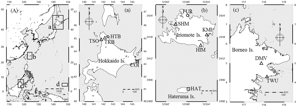
Fig. 1.

Land-use percentages for forest, farmland, water and urban areas were 74, 23, 2 and 1% in the northern part of Hokkaido, respectively (Hokkaido Prefecture, 2014); for Iriomote Island, these values were 94, 3, 2 and 1%, respectively (Taketomi Town, 2010). The main species in the forest include Abies sachalinensis, which measure 8–24 m in height, in the northern part of Hokkaido (Teshio) (Takagi et al., 2015) and Castanopsis sieboldii in Iriomote (Aramoto et al., 1989). The Danum Valley Conservation Area (438 km²) on Borneo Island (Sabah, Malaysia) is covered by tropical rainforests with widely distributed Dipterocarpaceae as the dominant species, but oil palm fields are also distributed in the northeastern part of the island (Marsh and Greer, 1992; Reynolds et al., 2011).

The CO₂ observations collected by the CO₂ sonde and the continuous CO₂ measurement system were performed at Teshio (TSO), Toikanbetsu (TKB) and Hamatonbetsu (HTB) in Hokkaido, Haimi (HIM), Komi (KMI), Funaura (FUR),and Shirahama (SHM) in Iriomote, and Tawau (TWU) and Danum valley (DMV) in Borneo. Latitude, longitude, temperature and precipitation data for the sites are summarized in Table 1. In the case of Hokkaido (Japan), three sites were chosen in terms of the wind direction (i.e. from the west (upwind) to the east (downwind)). In the case of Iriomote Island, four sites corresponding to four directions (E, W, S and N) were selected. This allowed us to use two appropriate sites according to the wind direction for the sonde experiments in Iriomote. In these cases, we expected that we could calculate the forest flux using the difference of the profile between the upwind site and downwind site. On the other hand, because wind speed is extremely low at the Borneo sites, we could not expect to make such observations by way of using the wind flow. Therefore, we chose a forest site (Danum valley) and a non-forest site (Tawau) to compare the time series of CO₂ profiles and calculate the CO₂ flux there.

Table 1.

Summary of the observation sites used in this study.

Observation type ^a SitesLocation Latitude and longitudeAnnual mean (°C)Monthly minimum (°C)Monthly maximum (°C)Precipitation annual (mm)Altitude (m)STSOTeshioHokkaidoJapan44°52′35″N, 141°44′36″E6.6−5.619.59251C5STKBToikanbetsuHokkaidoJapan44°55′19″N, 142°01′25″E6.1−7.419.887714C45°03′21″N, 142°06′26″E110CHTBHamatonbetsuHokkaidoJapan45°07′30″N, 142°20′53″E5.8−6.619.11,02517SHIMHaimiIriomoteJapan24°15′45″N, 123°52′08″E23.718.228.62,08747C51SKMIKomiIriomoteJapan24°19′07″N, 123°54′26″E––––19C23CFURFunauraIriomoteJapan24°24′33″N, 123°48′32″E23.718.128.92,23131SSHMShirahamaIriomoteJapan24°21′37″N, 123°45′07″E––––11C15STWUTawauBorneoMalaysia4°18′58″N, 118°07′06″E27.126.727.52,46019C23SDMVDanum valleyBorneoMalaysia4°57′58″N, 117°48′15″E26.625.627.32,850166CDMVDanum valleyBorneoMalaysia4°58′49″N, 117°50′39″E493

a S and C indicate CO₂ sonde and continuous measurements, respectively.

Equipment

2.2.

CO₂ sonde

2.2.1.

Fig. 2a-1 shows a schematic of the CO₂ sonde (MCD-10, Meisei Electric Co., Ltd.). The CO₂ sonde consists of a balloon, a cutter for cutting the rope, a parachute, CO₂ sensor (NDIR, non-dispersive infrared absorption), two 10 L aluminium bags filled with CO₂ standard gases (approximately 380 and 430 ppm, respectively) (scale: NIES09 (Machida et al., 2009)), and a radiosonde (RS-06G, Meisei Electric Co., Ltd.). The sensor took measurements at 4.0 and 4.3 μm of the wavelength for the base IR line and CO₂ IR absorption, respectively, and the resolution of the measurements was 0.1 ppm. The total weight was about 2 kg. Helium gas (3700 L) was used to inflate the balloon. The balloon, parachute, cutter and CO₂ measurement component were combined into one and launched at a rising speed of 2–3 m s⁻¹ to an altitude of 10 km. The cutter was used to complete the observation phase and drop the CO₂ sonde at that time. The CO₂ sonde measured alternately outside air and two CO₂ standard gases through the elevation ascent process. In addition, location information (latitude, longitude and altitude), air pressure, temperature and relative humidity were measured by the radiosonde. The sampling air was dried by the dehumidifying device, which was located in front of the pump in the CO₂ sensor. Filters (SLHA033SS: 0.45 μm; Millipore Co., Ltd.) were installed at the front and back of the dehumidifying part. Details about the other parameters can be viewed at the product’s home page (http://www.meisei.co.jp/products/meteo/co2.html).

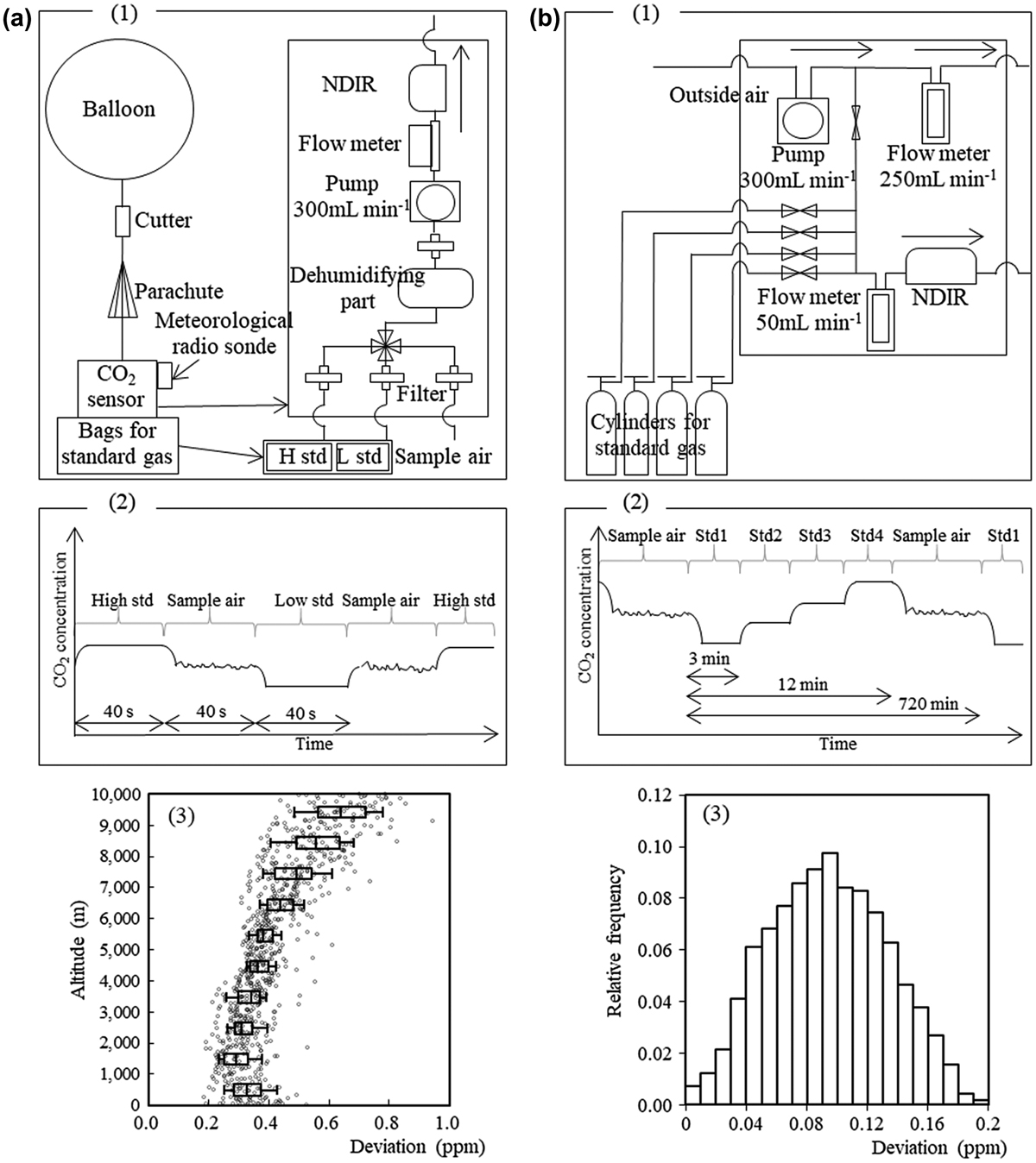
Fig. 2.

Fig. 2a-2 shows the measurement sequence of the CO₂ sonde. The CO₂ sonde measured the high CO₂ standard gas, outside air, low CO₂ standard gas and outside air for a duration of 40 s for each endpoint, and this sequence was repeated. The averaged standard deviation of the 40 s measurement signals for the CO₂ standard gas was 0.2–0.5 ppm from the ground to an altitude of 6000 m, and it was over 0.5 ppm from altitudes of 6000 m to 10,000 m (Fig. 2a-3); the measurement sensitivity decreased at higher altitudes because of the lower pressures in the absorption cell.

The observation dates are shown in Table 2. Sonde experiments were done at two sites simultaneously in each targeted forest area twice a day (at dawn just after sunrise and around 14:00). In the case of the Japanese sites (Hokkaido and Iriomote), two sites were chosen in terms of the wind direction (i.e. TSO (upwind) site and TKB (downwind) site). In Iriomote, we selected different combinations of the sites for the three measurements that were used to produce the final results. On the other hand, in Borneo, in order to evaluate CO₂ accumulation or absorption by the forest area, the differences of CO₂ profiles over time at a forest site (DMV) and non-forest site (TWU) were observed.

Table 2.

Location and time of the CO₂ sonde and continuous measurements.

Equipment ^a SitesDateHourSTSOHokkaidoJapan7 Sep 201205:00–06:26STKBHokkaidoJapan7 Sep 201205:00–06:24STSOHokkaidoJapan7 Sep 201214:00–15:30STKBHokkaidoJapan7 Sep 201214:00–14:41SHIMIriomoteJapan25 Sep 201314:00–15:30SSHMIriomoteJapan25 Sep 201314:00–15:30SHIMIriomoteJapan26 Sep 201306:00–07:43SSHMIriomoteJapan26 Sep 201306:00–07:21SKMIIriomoteJapan28 Sep 201314:00–15:29SSHMIriomoteJapan28 Sep 201314:00–15:29STWUBorneoMalaysia4 Aug 201514:00–15:19SDMVBorneoMalaysia4 Aug 201514:00–15:20STWUBorneoMalaysia5 Aug 201507:00–08:20SDMVBorneoMalaysia5 Aug 201507:00–08:20STWUBorneoMalaysia5 Aug 201514:00–15:19SDMVBorneoMalaysia5 Aug 201514:00–15:19STWUBorneoMalaysia6 Aug 201507:00–08:20SDMVBorneoMalaysia6 Aug 201507:00–08:21CTSOHokkaidoJapanAug 2012–Sep 2013CTKBHokkaidoJapanAug 2012–Mar 2017CHTBHokkaidoJapanAug 2012–Sep 2013CHIMIriomoteJapanJul 2013–Dec 2015CKMIIriomoteJapanJul 2013–Dec 2015CFURIriomoteJapanJul 2013–Dec 2015CSHMIriomoteJapanJul 2013–Dec 2015CTWUBorneoMalaysiaJan 2015–Mar 2017CDMVBorneoMalaysiaJan 2015–Mar 2017

a S and C indicate CO₂ sonde and continuous measurements, respectively.

The CO₂ sonde experiment was started in Hokkaido (typical northern Japanese forest) in September 2012. Next in 2013, we selected the subtropical forest (Iriomote) for the experimental site and the sonde experiments were launched on September 2013. Finally, we attempted the sonde experiments in Danum valley forest and Tawau on Borneo Island in August 2015 in cooperation with the Tawau Malaysian Meteorological Department (MMD).

Continuous CO₂ measurement equipment

2.2.2.

Fig. 2b-1 shows a schematic of the continuous CO₂ measurement system. The system consists of a pump, NDIR (Li-840A, Li-COR Co., Ltd.), a flow metre, and 10 L cylinders of CO₂ standard gases (approximately 370, 390, 410 and 430 ppm) (scale: NIES09). The inlets of TKB in Hokkaido and DMV in Borneo were installed at the observation towers (heights of 30 and 60 m from the ground, respectively), which are located about 5 km away from the site where we launched the CO₂ sonde. The DMV site was the Malaysian WMO monitoring site, which is located at the top of the mountain (430 m in altitude). The inlets of the other sites were installed on the roof or wall (approximately 4 m from the ground) of the buildings where the instruments were installed.

Fig. 2b-2 shows the measurement sequence of the continuous CO₂ measurement system. The system measured four kinds of CO₂ standard gas for 3 min each, and then, outside air was measured for 11 h and 48 min and this sequence was repeated. This system has no drying component, but the dry air based CO₂ mole fraction was calculated from the H₂O concentration by the Li-840A. Estimated accuracy for the sample air measurements was about 0.3 ppm, even though the accuracy for CO₂ standard gas was around 0.1 ppm (Fig. 2b-3).

The continuous CO₂ measurement system observed atmospheric CO₂ concentrations on the ground at three sites from August 2012 to September 2013 in Hokkaido, four sites in July 2013–December 2015 in Iriomote, and two sites in January 2015 to present in Borneo (Table 2).

Results and discussion

3.

Measurements by the CO₂ sonde

3.1.

Flight paths for the horizontal direction

3.1.1.

The horizontal pathways of the flights for each CO₂ sonde every 10 min are shown in Fig. 3. The CO₂ sondes launched from TSO and TKB in Hokkaido flew towards the east–north-east, and the sonde launched from TSO passed over TKB after 30 min and arrived at the sea after 60 min (Fig. 3a). The three CO₂ sondes launched from SHM in Iriomote were always driven out to the sea by the west–south-west wind from the land over a very short period of time. The two CO₂ sondes launched from HIM were also driven out to the sea rapidly. The CO₂ sonde launched from KMI crossed over the island from east to west after 30 min because of the wind from the ocean, and then, it flew towards the north-east (Fig. 3b). The CO₂ sondes launched from TWU and DMV in Borneo on all days flew to the north-east (Fig. 3c). Horizontal distances of sonde trajectories were shorter in Borneo than those in Japan because of the weaker horizontal winds in the tropics.

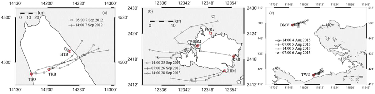
Fig. 3.

The sites TSO and TKB in Hokkaido on 7 September 2012, and KMI and SHM in Iriomote on 28 September 2013 were regarded as the upwind sites and downwind sites, respectively. HIM and SHM in Iriomote on 25 and 26 September 2013 also exhibited a relationship of an upwind site and downwind site for the Iriomote forest because HIM and SHM received unaffected and affected air masses from the forest, respectively. Although TWU and DMV in Borneo had no relationship indicative of an upwind site and downwind site, TWU was mainly influenced by the air over the sea and DMV was mainly influenced by the air over the forest.

Thus, we were able to confidently classify the experimental sites into upwind sites (U) and downwind sites (D) over the forests for Hokkaido and Iriomote as shown in Table 3. We could also classify TWU and DMV in Borneo as the coast site (C) and forest site (F), respectively, according to the sonde trajectories.

Table 3.

The height of the stable boundary layer (SBL) and convective planetary boundary layer (CBL) and average CO₂ concentrations inside the SBL and CBL.

SiteType ^a DateHourSBL and CBL height ^b Average CO₂ concentration ^c ΔCO₂ ^d (m)(ppm)(ppm)TSOHokkaidoU7 Sep 201205:00400387.0TKBHokkaidoD7 Sep 201205:00400391.64.5TSOHokkaidoU7 Sep 201214:001500384.9TKBHokkaidoD7 Sep 201214:001500384.4−0.5HIMIriomoteU25 Sep 201314:001000394.9SHMIriomoteD25 Sep 201314:001000393.9−1.0HIMIriomoteU26 Sep 201306:00200395.1SHMIriomoteD26 Sep 201306:00200395.70.5KMIIriomoteU28 Sep 201314:001000394.9SHMIriomoteD28 Sep 201314:001000393.5−1.4TWUBorneoC4 Aug 201514:001100403.3DMVBorneoF4 Aug 201514:002400396.6−6.7TWUBorneoC5 Aug 201507:00400411.4DMVBorneoF5 Aug 201507:00500434.823.4TWUBorneoC5 Aug 201514:001700403.8DMVBorneoF5 Aug 201514:001700397.8−6.0TWUBorneoC6 Aug 201507:00400416.6DMVBorneoF6 Aug 201507:00500442.025.4

a U, D, C and F indicate the upwind site, downwind site, coast site and forest site, respectively.

b We considered both the maximum vertical gradient of potential temperature and the minimum vertical gradient of specific humidity for the determination of the SBL and CBL height.

c CO₂ concentrations were averaged within the SBL and CBL.

d Differences in the CO₂ concentration between the downwind site and upwind site, or the forest site and coast site.

The height of the planetary boundary layer (SBL and CBL) and weather conditions

3.1.2.

Fig. 4 shows the potential temperature (PT) and specific humidity (SH) of vertical profiles from the ground to 4000 m in altitude at dawn and daytime at all sites. In addition, the SBL and CBL heights, which were presumed from the level of the maximum vertical gradient of potential temperature and the minimum vertical gradient of specific humidity, are shown in Table 3 and Fig. 4.

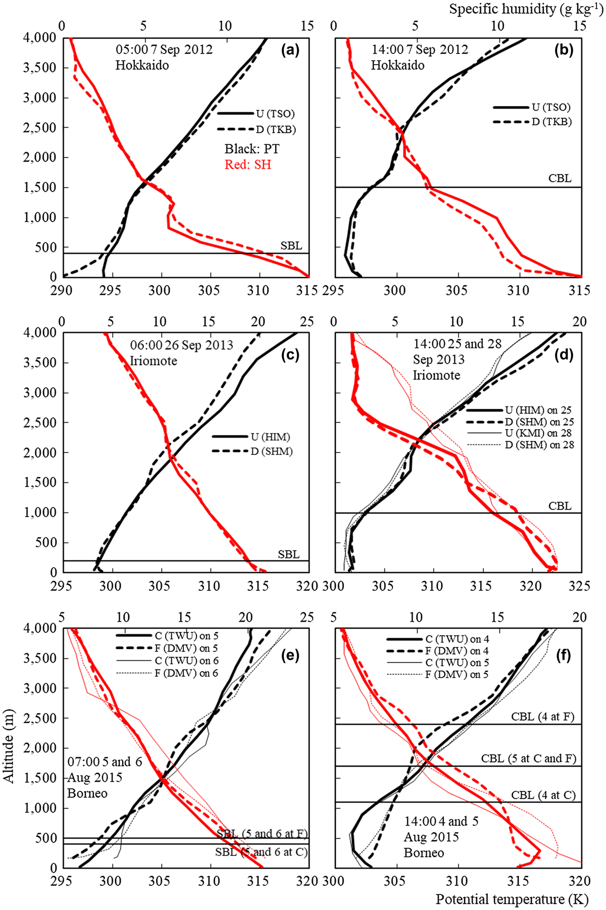
Fig. 4.

On Hokkaido and Iriomote Island, SBL and CBL heights for the upwind sites and downwind sites were almost the same. They were 400 m (SBL) at dawn and 1500 m (CBL) at daytime in Hokkaido, and 200 m (SBL) at dawn and 1000 m (CBL) at daytime in Iriomote.

Weather conditions were sunny on all days at both sites expect for at dawn on 26 September in Iriomote, which was partly cloudy. The wind speed in Hokkaido was 4 m s⁻¹ at dawn and 12 m s⁻¹ in the daytime. The wind speed in Iriomote was 6 m s⁻¹ on 25 and 26 September and 3 m s⁻¹ on 28 September; these values were slightly higher than usual because of the influence of a typhoon in the Pacific.

In the case of Borneo, SBL and CBL heights for the forest site (DVM) were a little higher than those at the coastal site (TWU) both at dawn and during the daytime on 4 August. Because 4 August 2015 was clear in the forest area, the CBL heights were relatively higher (2400 m) than those on 5 August (1700 m), when it was partly cloudy. The CBL heights of TWU and DMV on 5 August were the same. Air over TWU may have been affected by the inland forest at that time. The SBL heights at dawn were 400 m in TWU and 500 m in DMV. Wind speeds at both sites were approximately 0.2–0.5 m s⁻¹ at dawn and 0.8–1.2 m s⁻¹ during the daytime, and the wind speed in TWU was a little stronger (0.3–0.5 m s⁻¹) than that in DMV.

According to Wofsy et al. (1988), the SBL was reported to be about 300 m in the early morning in the Amazon forest area. Because DMV is a valley, the apparent SBL height may have been higher than that for the case of a flat plane forest. But as explained in the next section, this height of the boundary layer was consistent with the CO₂ concentration profile.

CO₂ vertical profiles

3.1.3.

Fig. 5 shows vertical CO₂ profiles from the ground to 4000 m in altitude and the SBL and CBL heights in Hokkaido (a and b), Iriomote (c and d), and Borneo (e and f) at dawn (a, c and e) and during the daytime (b, d and f). CO₂ data and altitude data were adopted as average values for the period when CO₂ sondes measured the sample air for 40 s. So, the data were plotted at intervals of 200–300 m.

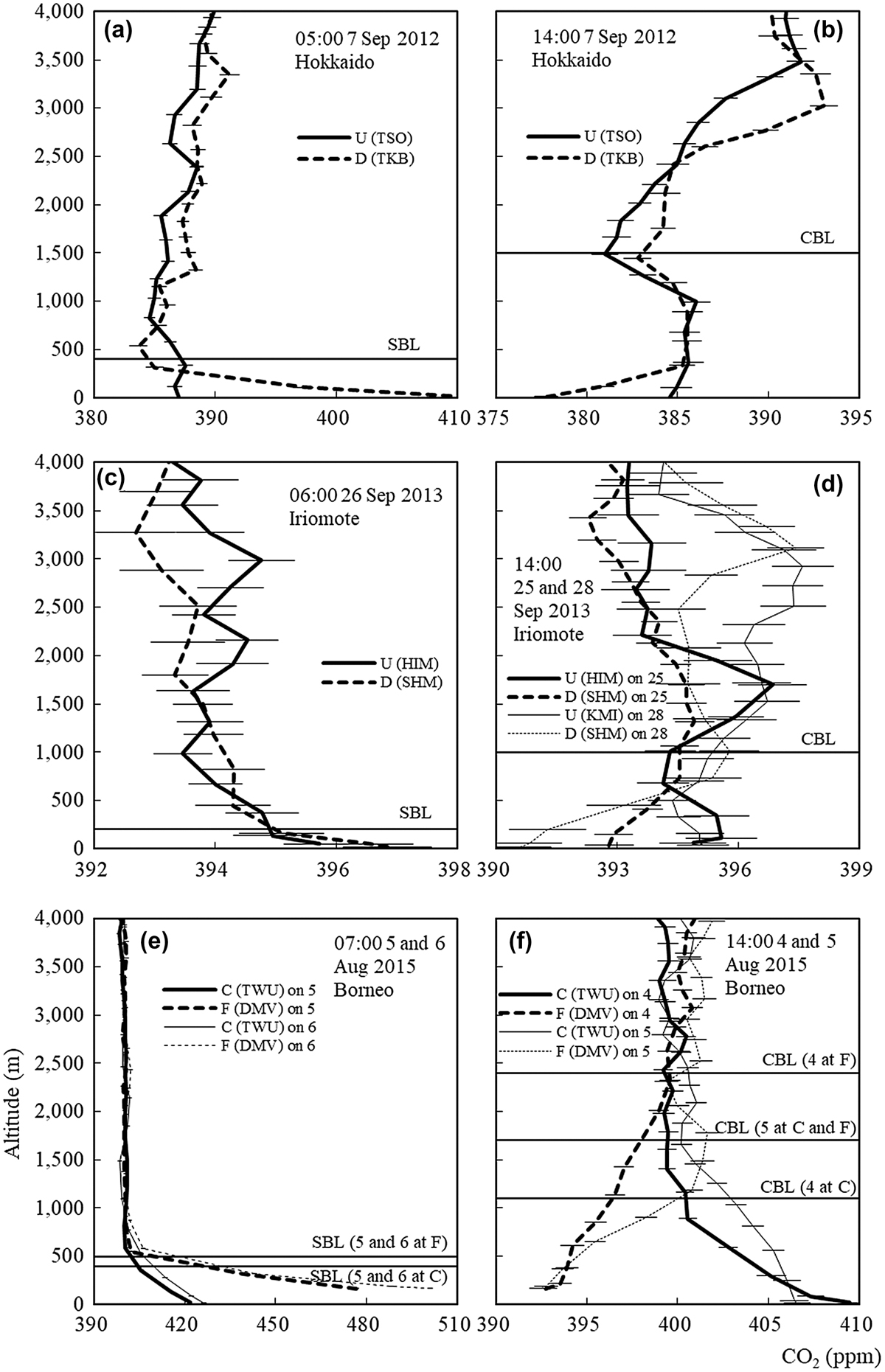
Fig. 5.

Hokkaido

3.1.3.1.

At dawn in Hokkaido (Fig. 5a), CO₂ concentrations inside the SBL at the downwind site showed relatively higher values than those above the SBL, while the CO₂ concentrations inside the SBL at the upwind site were almost the same as those above the SBL. At daytime in Hokkaido (Fig. 5b), the vertical profile of CO₂ showed lower concentrations below 500 m at only the downwind site. This was a major signal of the forest sink in the daytime along the air mass pathway from east to west.

We could recognize that the CO₂ profile had another low concentration layer from the CBL height (1500 m) to 3000 m at both the upwind site and the downwind site. It seemed that air above the CBL and air just below the CBL had mixed somewhere. However, this signal mainly existed above the CBL and both sites had a similar layer. So, the low CO₂ layer from 1500 to 3000 m might have been influenced by the regional Siberian forest sink, as derived from the trajectory analysis showing that the air mass originated from Siberia (data not shown).

Iriomote

3.1.3.2.

At dawn in Iriomote (Fig. 5c), CO₂ inside the SBL at both the upwind site and downwind site showed relatively higher concentrations than those above the SBL. Furthermore, the concentration inside the SBL at the downwind site was 1 ppm higher than the concentration at the upwind site, thus demonstrating the outflow of CO₂ from the island. At daytime in Iriomote (Fig. 5d), CO₂ concentrations inside the CBL at the downwind site on both 25 and 28 September showed decreasing profiles with altitude from the CBL height to the ground, while the concentrations at the upwind site showed no such profile. Yamamoto et al. (1996) reported on the distribution of CO₂ concentrations around Iriomote Island using a small air plane and found that the difference in concentrations between the upwind area and downwind area at a certain level (200–1000 m) were 2–4 ppm, which was almost the same level as our sonde observation.

On both days, weather was rather unstable because there was a small typhoon located in the Pacific several hundreds of kilometers away from the island. Therefore, the CO₂ profile seemed unclear above the CBL. Relatively large variation was detected, despite the fact that the precision of the CO₂ sonde was estimated to be about 1 ppm at higher altitudes such as 2000 m. As seen in the profile of SHM in Fig. 4d, the structure of air layers on 25 September was different from that on 28 September. In the case of 25 September, free tropospheric air came down to 2500 m and another layer existed in the region between the CBL (1000 m) and 2500 m, but on 28 September, air at the lower altitude seemed to be lifted up to 4000 m by the typhoon. However, such differences above the CBL were not taken into consideration during the calculation of the surface CO₂ flux because our measurements (within 1 h) were considerably shorter than such regional climatic phenomena.

Borneo

3.1.3.3.

At dawn in Borneo (Fig. 5e), CO₂ inside the SBL at both the coast site and the forest site on both 5 and 6 August showed a strong accumulation trend for CO₂ near the ground. Especially, the CO₂ concentrations at the forest site were 60–80 ppm higher inside the SBL than those at the coast site. At daytime in Borneo (Fig. 5f), CO₂ inside the CBL at the forest site on both August 4 and 5 was about 6 ppm lower than the concentration above the CBL, which suggests that the tropical rain forest can absorb CO₂ very strongly during the daytime. On the other hand, the CO₂ on the ground at the coast site displayed rather higher concentrations compared to those at higher levels even in the daytime.

The CO₂ concentrations inside the CBL at the downwind sites and the forest sites in Hokkaido, Iriomote and Borneo were always lower during the daytime and higher at dawn than those above the SBL, as well as those inside the CBL at the upwind sites or at the coast site. The difference in the averaged CO₂ concentration inside the CBL between the coast site and the forest site of Borneo during the daytime was 6.4 ppm, which was much higher than the difference between the upwind site and the downwind site of Hokkaido (0.5 ppm) and Iriomote (1.2 ppm) (Table 3). In addition, the coast and forest site difference for the averaged CO₂ concentration inside the SBL above Borneo at dawn was 24.4 ppm, which was much larger than the differences at Hokkaido (4.5 ppm) and Iriomote (0.5 ppm).

Chou et al. (2002) reported that atmospheric CO₂ concentrations in the vicinity of the ground in the forest at dawn and daytime were relatively higher and lower respectively than the upper air. Wofsy et al. (1988) found that CO₂ concentrations from the ground to an altitude of 1500 m over the forest were approximately 5 ppm lower than those over the ocean in daytime, while CO₂ concentrations above 1500 m over the forest and ocean showed no difference.

In the case of Hokkaido, the observed air masses were considered to pass across the forest that was distributed between the upwind site and the downwind site because the CO₂ sonde launched from the upwind site passed through the downwind site after 30 min (Fig. 3). The differences in CO₂ concentration between the upwind site and the downwind site were presumed to be caused by photosynthesis and respiration of the forest, as there was little influence from anthropogenic emissions.

On the other hand, in Borneo, the differences in the CO₂ concentration between dawn and daytime and between the coast site and the forest site reflect the influence from vertical mixing of the air, and the atmospheric transport for the horizontal direction was presumed to be very small (monthly averaged wind speed near the ground at these sites was approximately 1 m s⁻¹). However, at the coastal area (Tawau airport area, where there is no forest, only some vegetation cover on the ground), there seemed to be slight CO₂ emissions even in daytime.

Measurements by the multi-site continuous CO₂ monitors

3.2.

CO₂ daily variation on the ground during the observation periods of the CO₂ sonde experiments

3.2.1.

Hourly averaged CO₂ concentrations and hourly wind directions on the ground at the three sites around the date when we launched the CO₂ sondes (Hokkaido: 6–8 September 2012, Iriomote: 25–28 September 2013, Borneo: 4–6 August 2015) are shown in Fig. 6. The footprint size of each site was estimated at about 10–50 km in diameter from the wind speed. CO₂ data from the reference sites were also plotted in this figure so that comparisons could be made to the CO₂ concentrations in daytime when the air was well mixed.

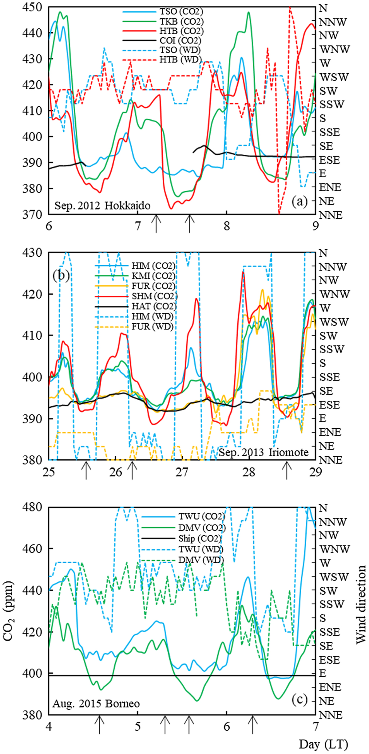
Fig. 6.

Hokkaido

3.2.1.1.

The CO₂ daily variation at TSO in Hokkaido was fairly small, while variation at the inland site TKB was relatively large (Fig. 6a). Because TSO was always the upwind site during the sonde observations and the wind came from the Sea of Japan, we observed maritime air at TSO and the CO₂ concentration was considerably stable. CO₂ concentrations on 6 and 8 September at TSO seemed to be very similar to the CO₂ concentrations at COI. Therefore, CO₂ concentrations observed at TSO could be treated as the regional background level.

On the other hand, since TKB and HTB were always the downwind sites during 6–7 September, CO₂ concentrations varied here because of the influence of the forest along the air pathways. These data showed lower concentrations in daytime than those at TSO. It is reasonable that HTB had much lower concentrations than TKB because HTB exhibits a longer distance over the forest sink along the wind pathway than TKB. Sonde experiments also showed similar CO₂ concentrations to the continuous measurements at the ground level at both the TSO and TKB sites.

Iriomote

3.2.1.2.

CO₂ concentrations in daytime at HIM and KMI in Iriomote Island were almost the same as those of the reference site HAT, which displayed approximate background concentrations over this region, while the SHM site showed about 5 ppm lower concentrations than those of HAT; the FUR site also showed lower concentrations, especially on 28 September (Fig. 6b). This was because the background maritime air came from the E–SE direction on this particular day, while the air masses over FUR and SHM seemed to have been influenced by the forest. Such a relationship was consistent with the sonde experiments.

CO₂ concentrations increased throughout the night from sunset to dawn at all sites, even at the upwind sites, because the total surface wind became weak at sunset and land breezes probably carried the air containing the land respiration signal. However, if we look closely at the data from midnight to morning, the concentrations at night in the downwind sites (FUR and SHM) were relatively higher than those in the upwind sites (HIM and KMI). Interestingly, CO₂ in SHM, which is an outlet site for the wind, showed much slower decreasing rates in concentrations after sunrise than those at the other sites, as if accumulated CO₂ over the island was swept away with the dominant wind, and at the same time, the concentration decreased towards afternoon through the forest sink process and the vertical mixing of the air. However, the upwind sites (HIM and KMI) showed sudden decreases in CO₂ concentrations to background levels with the change of wind direction and no change after that until sunset.

Borneo

3.2.1.3.

In the case of the Borneo site, CO₂ concentrations were monitored at TWU and DMV. At DMV, the continuous monitoring site and sonde experimental site were slightly different, as mentioned in the experimental section. As a result, we may have taken air at a little higher level than SBL at DMV.

As seen in Fig. 6c, CO₂ concentrations on 4–5 August at the TWU site in the daytime were generally 6–10 ppm higher than the background level in the Pacific taken by the ship observations. Such a CO₂ built-up phenomenon at the surface level was also seen in the sonde experiment, as shown in Fig. 5f. However, the CO₂ concentration on 6 August at the TWU site in the daytime was similar to the background level because the oceanic air came from the ocean side.

The DMV forest site showed considerably lower concentrations on 4–6 August in daytime, thus suggesting that the tropical rain forest can strongly uptake CO₂ from the air. This concentration decrease (7–12 ppm) was almost the same as the level observed by the sonde experiment. On the other hand, because the air sampling height at DMV was relatively higher (490 m) than that at the other site and the altitude was almost same as SBL, strong accumulation (e.g. over 100 ppm) of CO₂ in SBL, which was observed in the sonde experiment, could not be observed.

The coastal sites where the CO₂ daily variation was relatively small or the CO₂ concentration during the daytime was almost the same as that at the reference (background) site were all locations that were influenced by air masses from the ocean (TSO, HIM, KMI and TWU). On the other hand, the sites where the CO₂ daily variation was relatively large or the CO₂ concentration during the daytime was lower than that at the reference site (TKB, HTB, FUR, SHM and DMV) were influenced by the forest CO₂ sinks and emissions. Therefore, with results from measurements of the diurnal variation by ground-based continuous CO₂ monitors at multiple sites, we were largely able to see the forest sink signals by looking at the wind direction and comparing the CO₂ levels in daytime to those at regional reference (background) sites. This method is very simple for detecting the forest sink signals in comparison to vertical profile measurements.

The general relationship between CO₂ and wind direction according to the observations collected over several years

3.2.2.

To generalize the forest photosynthesis signal in terms of the air CO₂ signal observed at the ground sites, we calculated the ΔCO₂, which is the difference in CO₂ concentration from the background site at 14:00; furthermore, we confirmed the relevance of the ΔCO₂ and the wind direction at the site. The average ΔCO₂ values during the daytime (14:00) for the observation periods (Hokkaido: August–September 2012 and July–September 2013, Iriomote: July–September 2013, 2014 and 2015, Borneo: July–September 2015) are shown in Fig. 7, and data were classified into four wind direction categories (north = NW–N–NE, south = SE–S–SW, east = NE–E–SE and west = SW–W–NW).

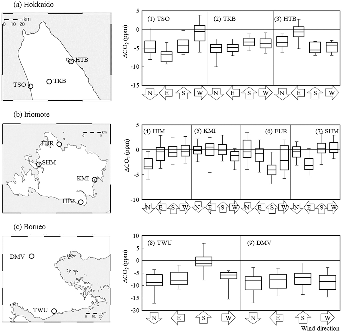
Fig. 7.

The data for ΔCO₂ in Hokkaido are shown in Fig. 7a. The ΔCO₂ for TSO showed negative values when the wind direction was north, east and south, while the ΔCO₂ was about zero when the wind direction was west. The ΔCO₂ for TKB showed negative values in all wind directions. The ΔCO₂ for HTB showed negative values when the wind direction was north, south and west, and it was about zero when the wind direction was east. Thus, it seemed to be a general rule that ΔCO₂ was about zero when the wind (or air mass) came directly from the sea and ΔCO₂ was always negative when the wind (or air mass) passed over the forest in northern Hokkaido. Additionally, the ΔCO₂ of TKB, which is located in the inland forest area, showed negative values regardless of the differences in wind direction.

The data for ΔCO₂ in Iriomote and Borneo are shown in Fig. 7b and c, respectively. Both sites had the same observational results as were seen in the case of northern Hokkaido. In the case of Iriomote, four sites clearly showed reasonable differences in the wind direction for the negative case. In the case of TWU in Borneo, large negative values were seen in the cases of north, east and west wind directions, but not for the south direction. For DMV, ΔCO₂ during the daytime was always negative.

Thus, the observation network on the ground, which consists of continuous CO₂ measurement equipment at multiple sites around the forest, was able to capture the phenomenon of about 1–10 ppm decreases in atmospheric CO₂ concentrations during the daytime at the surface level caused by photosynthesis of the forest. The differences in CO₂ concentration between the upwind site and the downwind site in Hokkaido and Iriomote occurred because of photosynthesis and respiration of the forest along the flight path from the upwind site to the downwind site (Fig. 3). Therefore, theoretically speaking, the average CO₂ flux of the forests could be calculated from the differences in CO₂ concentration between the upwind site and the downwind site, the wind conditions, and some estimation of the vertical profile from the SBL and CBL height.

Estimation of the CO₂ flux from vertical profile data

3.3.

On the basis of observational results for CO₂ vertical profiles collected by CO₂ sondes and CO₂ concentrations on the ground collected by continuous CO₂ measurements, the differences in CO₂ concentrations between the upwind site and the downwind site represent the influence of the forest between the two sites. First, we calculated the average CO₂ flux of the forest in Hokkaido and Iriomote by Equation (1) based on the box model shown in Fig. 8a. This model calculates the CO₂ flux from the differences in CO₂ concentrations between the upwind site and the downwind site as follows:

(1)

$$F=\frac{{\sum }_{i=1}^m[{\rho }_i{\text{DC}}_i({\text{Dh}}_i-{\text{Dh}}_{i-1})]-{\sum }_{i=1}^n[{\rho }_i{\text{UC}}_i({\text{Uh}}_i-{\text{Uh}}_{i-1})]}{\text{Dis}WS}$$

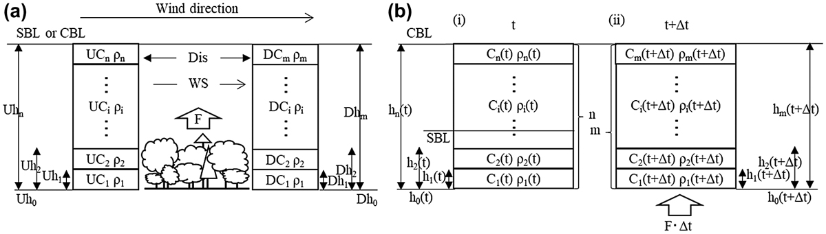
Fig. 8.

Here, F is the CO₂ flux (μmol m⁻² s⁻¹); UC _i and DC _i are the CO₂ concentrations (ppm) of the i-th layer of the vertical profiles at the U (upwind) site and D (downwind) site, respectively; and Uh _i and Dh _i are the height (m) of the i-th layer where UC _i and DC _i were measured, respectively. Furthermore, ρ _i is the molar air density (mol m⁻³) in the i-th layer. The planetary boundary layer (PBL) heights (SBL or CBL) (m) are indicated as Uh _n and Dh _m for the upwind site and downwind site, respectively, which were usually the same in our case, as shown in Table 3. However, because the data interval in terms of height was a little different for each observation, we used a different layer number for the CO₂ profiles at the U-site and D-site (i.e. n and m). WS is the average wind speed in the SBL or CBL (m s⁻¹), which was calculated from the flight distance of the CO₂ sonde. Dis is the distance (m) between the upwind site and downwind site.

For TWU and DMV in Borneo, the differences in CO₂ concentrations between dawn and daytime were assumed to occur only as result of photosynthesis and respiration of the forest around each site because TWU and DMV did not have an upwind site and downwind site relationship as did the Japanese sites (Fig. 3); moreover, the average wind speed was very weak (only 1 m s⁻¹). The average CO₂ flux in Borneo was calculated by Equation (2) based on the box model in Fig. 8b), which was created on the basis of Culf et al. (1997) from the differences in CO₂ concentrations between dawn and daytime as follows:

(2)

$$F=\frac{{\sum }_{i=1}^m[{\rho }_i(t+\mathrm{\Delta }t)C_i(t+\mathrm{\Delta }t)(h_i(t+\mathrm{\Delta }t)-h_{i-1}(t+\mathrm{\Delta }t))]-{\sum }_{i=1}^n[{\rho }_i(t)C_i(t)(h_i(t)-h_{i-1}(t))]}{\mathrm{\Delta }t}$$

Here, F is the CO₂ flux (μmol m⁻² s⁻¹); C _i (t) and C _i (t + ∆t) represent the CO₂ concentration (ppm); h _i (t) and h _i (t + ∆t) are the height (m) of the i-th layer at the moment of time t and t + ∆t, respectively; h _n (t) is the same as h _m (t + ∆t), corresponding to either the CBL height (m) at a time of t or t + ∆t (Table 3); ρ _i (t) and ρ _i (t + ∆t) are the molar air density (mol m⁻³) at that moment; and ∆t is 7 h (from 07:00 to 14:00) or 17 h (from 14:00 to 07:00) (s). In this case, flux F is the average value during ∆t.

The estimated CO₂ fluxes of the forests in Hokkaido, Iriomote and Borneo are summarized in Table 4. The CO₂ flux at dawn and daytime were 11.8 and −14.4 (μmol m⁻² s⁻¹) in Hokkaido, and 3.9 and −11.8 to −15.0 (ave: −13.4) in Iriomote, respectively. The CO₂ fluxes from daytime to the next dawn and from dawn to daytime in Borneo were 3.2 to 4.0 (ave: 3.6) and −10.3 at TWU (coast site) and 16.0 to 16.9 (ave: 16.5) and −37.7 at DMV (forest site), respectively. We also calculated the CO₂ flux for layers from the surface to the SBL and CBL height + 100 m in altitude and from the surface to the SBL and CBL height – 100 m (Table 4). The values of CO₂ flux changed 46% in Hokkaido, 36% in Iriomote and 6% in Borneo when the SBL and CBL height changed ± 100 m. The values in Hokkaido and Iriomote were largely dependent on the SBL and CBL height.

Table 4.

Estimated CO₂ flux in the three forests.

SiteTimeCO₂ fluxμmol m⁻² s⁻¹DateHourMean ± SE ^a +100 m ^b −100 m ^c Hokkaido7 Sep 201205:0011.8 ± 0.410.713.3Hokkaido7 Sep 201214:00−14.4 ± 1.2−10.8−20.8Iriomote25 Sep 201314:00−15.0 ± 4.4−20.3−14.1Iriomote26 Sep 201306:003.9 ± 0.45.04.4Iriomote28 Sep 201314:00−11.8 ± 1.6−10.4−9.7TWUBorneo4–5 Aug 201514:00–07:003.2 ± 0.13.33.0DMVBorneo4–5 Aug 201514:00–07:0016.9 ± 0.216.816.9TWUBorneo5 Aug 201507:00–14:00−10.3 ± 0.2−10.8−10.0DMVBorneo5 Aug 201507:00–14:00−37.7 ± 0.3−38.4−37.6TWUBorneo5–6 Aug 201514:00–07:004.0 ± 0.14.13.4DMVBorneo5–6 Aug 201514:00–07:0016.0 ± 0.116.215.8

a Calculations for the SBL and CBL.

b Calculations for the layer from the surface to the SBL and CBL height + 100 m in altitude.

c Calculations for the layer from the surface to the SBL and CBL height – 100 m in altitude.

The values of CO₂ flux at dawn and daytime at all sites were positive and negative, respectively, and the absolute values at daytime were higher than those at dawn. The CO₂ flux of DMV in Borneo was 4 times higher than that at TWU. This may suggest that the atmosphere around the DMV site was strongly influenced by photosynthesis and respiration from the tropical rain forest. Furthermore, the CO₂ flux at DMV was approximately three times higher than that at Hokkaido and Iriomote, which is reflective of the relatively large density of biomass. This difference was fairly consistent with other data suggesting that the amount of biomass per unit area of Borneo is about 300 MgC ha⁻¹ (e.g. Saatchi et al., 2011), which is a value about three times larger than that in the northern Hokkaido region (about 80–100 MgC ha⁻¹ around TKB) (e.g. Takagi et al., 2015).

We compared our results in Hokkaido with the CO₂ flux measured by the eddy-covariance method around TKB (Takagi et al., 2009) on the same day (Fig. 9). The values for the CO₂ flux in this study were mostly the same as the values derived by the eddy-covariance method. Thus, our method, which involves measuring the differences in the vertical CO₂ profiles inside the SBL and CBL between an upwind site and downwind site using CO₂ sondes, can reasonably calculate the CO₂ flux for a region.

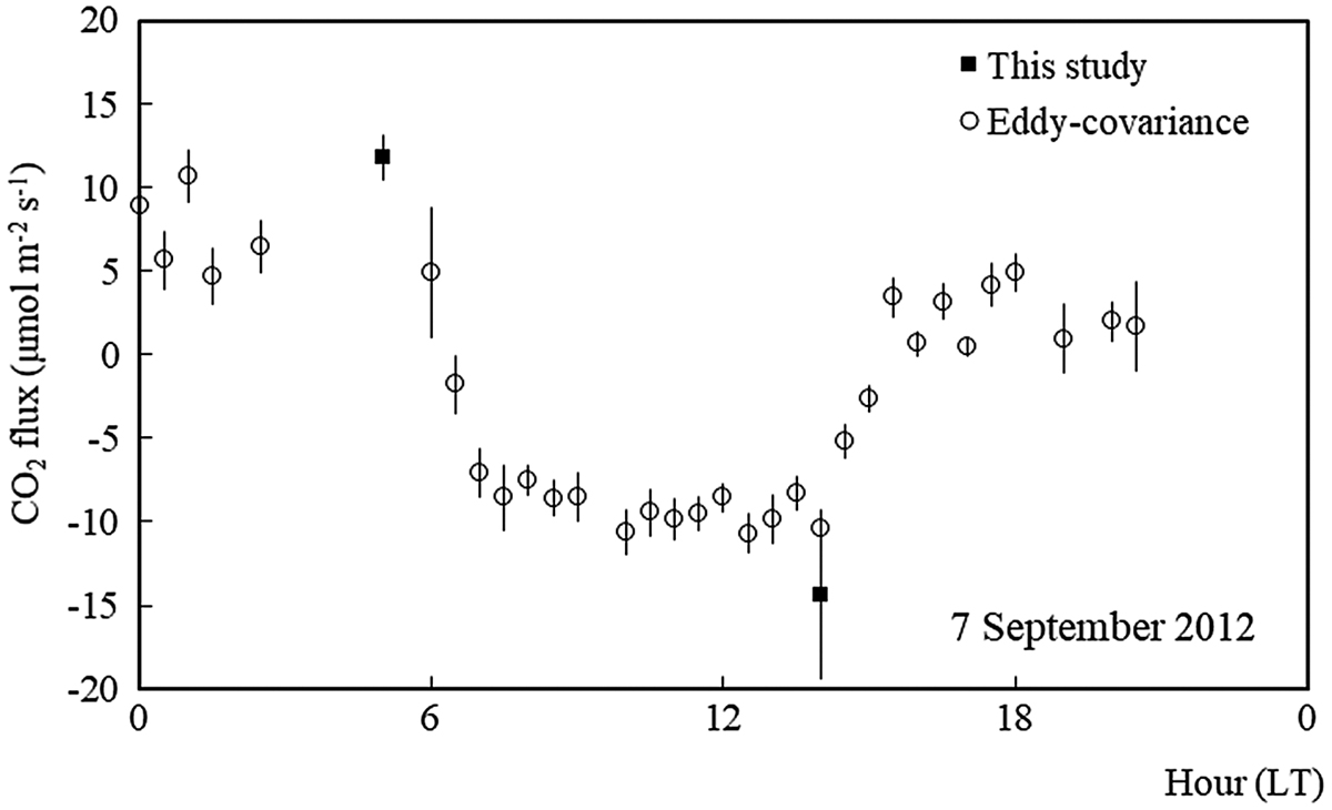
Fig. 9.

We also compared the CO₂ fluxes at Iriomote and Borneo obtained in this study with the previous flux data measured at the same or similar places (i.e. Iriomote, Amazon and Pasoh) (Fig. 10). Yamamoto et al. (1996) estimated the CO₂ flux from aircraft observations of CO₂ around Iriomote Island on March and November 1991 and July 1992 and reported that the CO₂ fluxes around 06:00 and around noon were 2.9 and −3.1 to −15.2 μmol m⁻² s⁻¹, respectively. Those values are almost the same as the values from our study (06:00: 3.9, 14:00: −11.8 to −15.0 μmol m⁻² s⁻¹) at the end of September in Iriomote. The CO₂ fluxes (μmol m⁻² s⁻¹) in August, which were measured by the eddy-covariance method in the Amazon (Wu et al., 2016) and Pasoh in the Malay Peninsula (Kosugi et al., 2008) were compared with the DMV’s CO₂ flux. Although note that the environmental conditions such as climate, vegetation type and carbon stocks (Gibbs et al., 2007) of the Amazon are different from those of Borneo. The CO₂ flux of DMV in Borneo at dawn showed a value of 16.0 to 16.9 (ave: 16.5) and these data were within the values of CO₂ fluxes in the Amazon (ave: 5.5, min: −6.6, max: 22.9) and Pasoh (ave: 4.9, min: −14.8, max: 28.1). The values of DMV’s CO₂ flux during the daytime (−37.7) were close to the minimum values of the CO₂ fluxes of the Amazon (ave: −13.5, min: −31.0, max: 1.3) and Pasoh (ave: −17.6, min: −35.4, max: 0.2). As a result, the CO₂ flux of DMV’s forest in this season is estimated to be almost the same or larger than the forest flux at the Amazon and Pasoh.

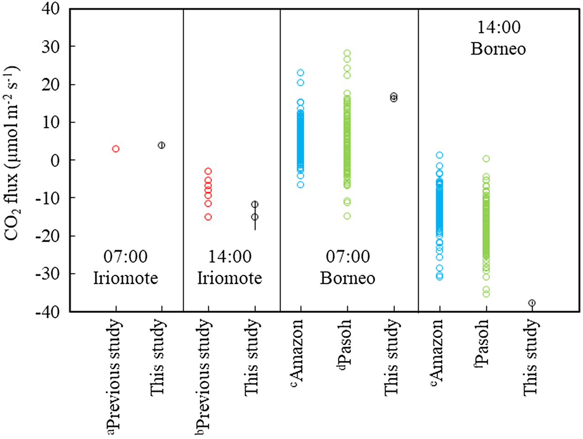
Fig. 10.

^aCO₂ flux at Iriomote from noon to 17:00 in March and November 1991 and July 1992 (Yamamoto et al., 1996). ^bSame as a but from 05:00 to 07:00 in July 1992. ^cHourly CO₂ flux at 05:00 in the Santarem-km67-Primary Forest, Amazon (latitude: 2°51′24.1″S, longitude: 54°57′32.0″W), in August from 2002 to 2011 (though data for 2006 and 2007 are not included) (Ameriflux, http://ameriflux.lbl.gov/data/download-data/). ^dHourly CO₂ flux at 06:00 on the Pasoh Forest Reserve, Malay Peninsula (latitude: 2°58′14.6″N, longitude: 102°17′57.8″E), in August from 2003 to 2009 (Asiaflux, https://db.cger.nies.go.jp/asiafluxdb/?page_id=16). ^eSame as c but for noon. ^fSame as d but for noon.

Therefore, it is apparent that the approximate value of the instant net CO₂ flux can be calculated by the differences in CO₂ concentrations obtained from measuring the vertical CO₂ profiles along upwind sites and downwind sites or along a time course such as from dawn to daytime in the tropical forest.

Conclusion

4.

We performed two types of observations in three different forests, which were, in Borneo Island, Hokkaido Island and Iriomote Island in the summers of 2012–2015. One method involved measuring vertical CO₂ profiles over the forest using CO₂ sondes, and the other method involved continuous measurements of surface CO₂ concentrations at multiple sites in and around the forest.

CO₂ sonde observations showed a clear signal from the effect of respiration and photosynthesis by the forest in the vertical CO₂ profiles at each site. Especially, the tropical rain forest of Borneo showed a large sink signal in the profile. For instance, average CO₂ concentrations in the SBL and CBL of the DMV forest site in Borneo at dawn and daytime showed values that were 24.4 ppm higher and 6.4 ppm lower than those at the coast site TWU, respectively. Meanwhile, the CO₂ concentrations of the downwind sites in Hokkaido and Iriomote at dawn and daytime were 0.5–4.5 ppm higher and 0.5–1.4 ppm lower, respectively, than those at the upwind sites, which suggests that the emission and uptake rates were relatively smaller than those in the tropical rain forest.

To confirm the signals of forest uptake and emission obtained by the sonde technology, we installed multiple continuous CO₂ measurement equipment in and around the forest and performed continuous observations of CO₂ concentrations on the ground in conjunction with the sonde observations. The sites that received oceanic air masses generally showed levels similar to regional background levels of CO₂. On the other hand, if the site was located downwind from the forest, a large daily variation was found corresponding to forest respiration at night and uptake during the daytime.

The findings for CO₂ concentrations around the forest showed systematic wind dependency. If we compared the CO₂ concentration at a site to the regional background level, forest uptake always decreased the CO₂ concentration at the downwind sites during the daytime to about 1–10 ppm lower than the background level values, while forest respiration increased the CO₂ concentration at night by about 20–30 ppm. In the case of Borneo, the investigated forest was so large in relation to the wind speed effects that the experimental sites were not located along the pathway of the air mass. However, we did see a large difference in the CO₂ daily variation between the forest site (DMV) and the coast site (TWU). Similarly, to other forests, coastal sites showed almost background CO₂ levels in daytime when the air came from the sea side, but the forest sites always showed 3–9 ppm lower concentrations than the Pacific background concentration in the daytime and with any wind direction. These findings indicate that the ground level CO₂ concentration can clearly show the forest CO₂ flux signal, and they also indicate that the CO₂ concentration always has a distinct local spatial distribution around the forest.

We estimated CO₂ fluxes in Hokkaido, Iriomote and Borneo from the differences of CO₂ vertical profiles between the sites or times according to the CO₂ sonde observations. CO₂ uptake (μmol m⁻² s⁻¹) during the daytime at the forest site in Borneo was −37.7, which was four times larger than that at the coast site (−10.3) of Borneo and three times larger than the rate at the forest in Hokkaido (−14.4) and Iriomote (−13.4). The CO₂ emission at dawn for the forest site in Borneo showed a value of 16.5, which was higher than that at the coast site (3.6) in Borneo, that in Hokkaido (11.8) and that in Iriomote (3.9). These values were compared with previously reported values obtained by other methods such as aeroplane measurements and the eddy-covariance method at similar locations including the Pasoh forest in Malay and the Amazon. We found that the flux estimated by the sonde observations in different types of forests showed good agreement with previous data.

Therefore, we concluded that sonde observations for vertical profile measurements over forest areas and additional multi-site CO₂ monitoring around the forest could provide fairy good flux estimations even in tropical rain forests. Sondes are relatively easy to operate and require small amounts of manpower compared to aircraft observations. Thus, this method should be valuable to use over relatively large regional forests. In future studies, it would be worthwhile to compare such sonde data to eddy-covariance flux measurements and inverse flux calculations over the same large regional forest tracts.

In the near future, usage of satellite CO₂ measurement data will likely become commonplace for regional CO₂ flux measurements, even for the MRV (measuring, reporting and verifying) activities associated with REDD+ efforts in many forested countries. From the results of this study, we could estimate that the CO₂ concentration in the PBL at daytime over the SE Asian tropical rain forest site was about 6–7 ppm lower than the background level because of photosynthesis by the forest, and this signal could be detected by satellite observations (i.e. GOSAT) even though this region is always covered by clouds. On the other hand, for Hokkaido (subarctic region) and Iriomote (subtropical region), the difference between the site and background was around 1 ppm, which will require higher analytical precision (<0.5 ppm), which is a target of GOSAT-2.

In the future, it will be important to use different kinds of techniques such as sondes, aircraft and satellites to evaluate regional forest fluxes, which are presently measured mainly by the eddy-covariance method. The sonde method will likely be the most effective for estimations of CO₂ flux measurements over tropical areas where satellite observations and aircraft measurements would be relatively difficult to collect.

Disclosure statement

No potential conflict of interest was reported by the authors.

Funding

This work was supported by funds (Development of Monitoring Technology Related to Global Warming) from the Ministry of the Environment, Japan.