
Introduction
1.
Gas fluxes between the soil and the atmosphere are highly relevant for the climate of the Earth (Ball, 2013). Large amounts of carbon dioxide, methane and nitrous oxide are emitted from the soil into the atmosphere (Smith et al., 2003; Vor et al., 2003). One factor governing the emission of greenhouse gases into the atmosphere is the soil gas transport. Commonly, it is assumed that soil gas transport is dominated by molecular diffusion (Maier and Schack-Kirchner, 2014). However, soil gas transport can also be altered through advection (Amos et al., 2009; Bowling and Massman, 2011). In addition, an enhancement of soil gas transport was observed during periods of high wind speed. This enhancement results from an advective–dispersive enhancement of soil gas transport in the soil pores through dynamic changes in the air pressure field above the soil and is referred to as wind-induced pressure pumping effect (Massman et al., 1997; Poulsen and Sharma, 2011; Maier et al., 2012). Well and deeply aerated soils are believed to be most susceptible to the pressure pumping effect (Maier et al., 2010, 2012).
Recent research at a conifer forest site showed that wind-induced air pressure fluctuations in a specific frequency range influence the topsoil gas transport (Mohr et al., 2016). Moreover, a pressure pumping coefficient (PPC, in Pa s−1) was derived, describing the strength of the pressure pumping. Based on 30 min intervals, a connection between PPC and the above-canopy wind speed was found. It was assumed that the observed air pressure fluctuations originate from air masses above the canopy, which would lead to time differences between signals measured at different heights. However, in their study no time lags between the air pressure signals at different heights were observed, leaving the origin of the air pressure fluctuations unclear. Thus, this study aims to find possible links between airflow characteristics and wind-induced air pressure fluctuations at the forest site, to investigate their spatial below-canopy variability and to describe the characteristics of pressure waves associated with air pressure fluctuations. Furthermore, it aims to determine the spatial variability of the pressure pumping effect.
Materials and methods
2.
Measurement site
2.1.
Airflow and air pressure measurements were conducted from 4 October 2016 to 24 November 2016 at the forest meteorological research site in Hartheim, Germany, located approximately 25 km to the south-west of Freiburg (47°56′N, 7°36′E). The forest at the research site is a single-layered plantation of Scots pine (Pinus sylvestris L.) with a mean tree height h of 18 m, a mean stand density of 580 trees ha−1 and a mean plant area index of 1.5. The soil at the research site is well-aerated and classified as Haplic Regosol after the world reference base for soil resources classification (FAO, 2015).
Airflow measurements
2.2.
Airflow at the research site was monitored by measuring the x- (u), y- (v), and z- (w) component of the wind vector (in m s−1) with ultrasonic anemometers (81000VRE, R.M. Young Company, Traverse City, MI, USA). Two measurement towers (T1, T2) separated by a distance of 40 m were used for the airflow measurements: T1 with a height of 30 m and T2 with a height of 18 m. The airflow measurement heights were 2 m (z 1/h), 9 m (z 2/h), 18 m (z 3/h), 21 m (z 4/h) and 30 m (z 5/h) at T1 and 18 m (z 3/h) at T2. The airflow data were recorded at a frequency of 10 Hz.
Air pressure measurements
2.3.
Piezo-resistive differential pressure sensors (GMSD 2.5 MR, Greisinger Electronic GmbH, Regenstauf, Germany) with a reference box were used for the air pressure measurements (Mohr et al., 2016). This system allows for measuring all air pressure fluctuations with frequencies >0.0005 Hz. Two measurement configurations were set up at the forest floor: Five pressure sensors (N, E, S, W, C) were aligned in an array between the two towers (Fig. 1a). The air pressure p (in Pa) measured halfway between the two towers was considered as the reference pressure p C measured at the center C of the sensor array. In addition, air pressure in a distance from C to the north (p N ), east (p E ), south (p S ) and west (p W ) was measured.
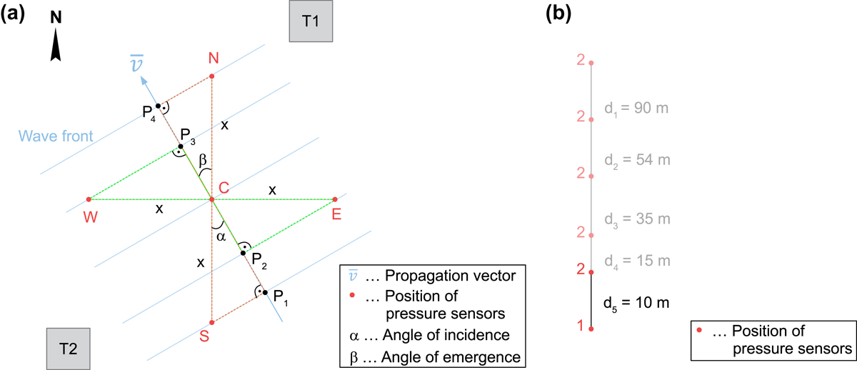
Fig. 1.
Schematic representation of the measurement configurations: (a) An array of five air pressure sensors installed between the towers T1 and T2. An arbitrary air pressure wave is shown in blue. The orange and green right-angled triangles are used to calculate the direction of propagation of the air pressure wave. (b) Two air pressure sensors installed with varying distance d i (i = 1, …, 5).
Two pressure sensors were used to evaluate the spatial variability of air pressure fluctuations, the distance d i (i = 1, …, 5) between the two sensors was gradually decreased from around 90 m to around 10 m (Fig. 1b).
The sampling frequency of air pressure was 2 Hz.
Data processing
2.4.
Data analysis was based on 30 min intervals. Relevant air pressure fluctuations were found to occur when mean above-canopy wind speed exceeds 1 m s−1, which is consistent with results from a previous study (Mohr et al., 2016). Therefore, all 30 min intervals with mean above-canopy wind speed lower than 1 m s−1 were excluded from further analysis.
Air pressure data
2.4.1.
All measured air pressure signals were filtered with a fourth order infinite impulse response band pass filter with lower and upper cutoff-frequencies of 0.01 Hz and 0.10 Hz. This frequency range was shown to be relevant for wind-induced pressure pumping (Mohr et al., 2016).
For the determination of the spatial variability of air pressure fluctuations, the cross-correlation function xcf was calculated between the filtered air pressure signals of two pressure sensors. The maximum value of xcf was used to specify the strength of cross-correlation between the two pressure signals.
Results reported by Mohr et al. (2016) demonstrate simultaneous occurrence of air pressure fluctuations at z 1/h to z 5/h. In contrast, results from trial experiments using transects of air pressure sensors at the forest floor showed the same air pressure fluctuations, but with clear time lags. Thus, it was inferred that the observed air pressure fluctuations propagate horizontally as a plane wave rather than vertically.
To determine the direction of propagation of the air pressure fluctuations, the time differences between p C and p N , p E , p S , and p W (, , , and ) were used. The time differences were specified using xcf. The order of observation of the air pressure fluctuations at each pressure sensor results from these time differences. Eight different orders are possible:
• Air pressure fluctuations propagating from northeastern (NE) to southwestern (SW) directions: NECWS and ENCSW.
• Air pressure fluctuations propagating from southeastern (SE) to northwestern (NW) directions: SECWN and ESCNW.
• Air pressure fluctuations propagating from southwestern (SW) to northeastern (NE) directions: SWCEN and WSCNE.
• Air pressure fluctuations propagating from northwestern (NW) to southeastern (SE) directions: NWCES and WNCSE.
Assuming a plane air pressure wave propagating from SE to NW, where the wave front is perpendicular to the direction of propagation, four different right-angled triangles can be used to calculate the angle of incidence (α, in °) and angle of emergence (β, in °) at C (cf. Fig. 1a). For both angles N is defined as 0°/360°, E as 90°, S as 180° and W as 270°. Ideally α is equal to β. However, a distinction between α and β was made to validate the developed methodology.
For α, first the triangle S-P1-C is considered:
The second equation for α is obtained from the triangle C-P2-E:
Dividing Equation (2) by Equation (1) leads to
Now that α is known, the propagation speed v α (in m s−1) of the inclining air pressure wave can be calculated:
Using triangles C-P3-W and N-P4-C, β and the propagation speed v β (in m s−1) of the emerging air pressure wave can be determined:
From α and β, and v α and v β , a mean direction of propagation (in °) and a mean propagation speed (in m s−1) was calculated (Berens, 2009).
These calculations were also done for the other possible propagation directions, leading to similar equations.
All 30 min intervals with a difference between α and β larger than 10° were excluded from further analysis (<10% of all 30 min intervals). This was necessary to assure a consistent calculation of , since large changes in propagation direction over a few metres were assumed to be implausible.
In addition, PPC which describes the strength of pressure pumping, was calculated (Mohr et al., 2016):
with the sampling frequency F s (in Hz), the number of pressure measurements N in a 30 min interval and the air pressure difference between two subsequent measurements (in Pa).
Airflow data
2.4.2.
Wind vector data were despiked (Mohr and Schindler, 2016) and the mean wind speed (in m s−1), mean horizontal wind speed (in m s−1) and the mean wind direction (in °) were calculated for all measurement heights (Berens, 2009).
Results and discussion
3.
Direction of propagation of air pressure fluctuations
3.1.
Figure 2 shows versus the mean above-canopy () and below-canopy wind direction ().
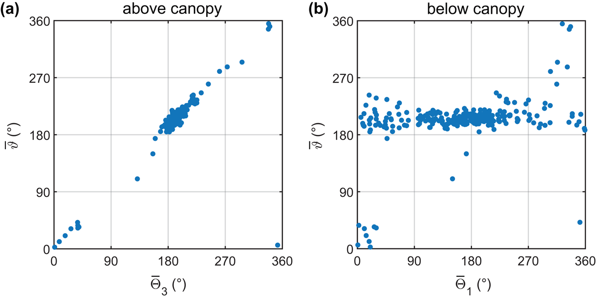
Fig. 2.
Dependence of mean direction of propagation of air pressure fluctuations () on (a) mean wind direction at z 3 () measured at T1, (b) mean wind direction at z 1 () measured at T1.
It is obvious that during the measurement period airflow from the south dominates. Only during a few intervals, northeastern and northwestern wind directions occur. It can be seen that strongly (coefficient of determination R 2 = 0.98) correlates to (Fig. 2a). Similar correlations can also be found for and . In contrast, the air pressure fluctuations do not seem to be connected to below-canopy airflow (Fig. 2b).
These results are in accordance with a previous study. Sigmon et al. (1983) who deduced the direction of propagation of air pressure fluctuations in a deciduous forest also reported that the fluctuations propagate in the same direction as the mean above-canopy wind direction.
Propagation speed of air pressure fluctuations
3.2.
Figure 3 shows an increase of with increasing and . Values of are in the order of (up to 6.5 m s−1). The strong correlation between and (R 2 = 0.83) indicates that there is a connection between the observed air pressure fluctuations at the forest floor and the above-canopy airflow. The connection between and is much less pronounced.
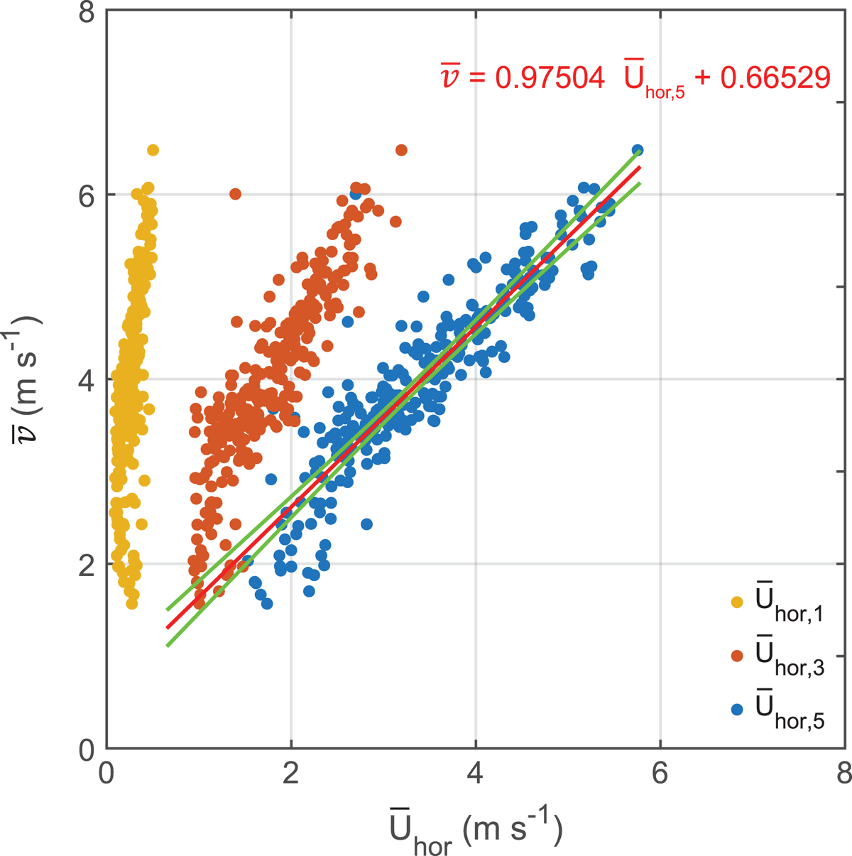
Fig. 3.
Dependence of mean propagation speed of the air pressure fluctuations () on mean horizontal wind speed at heights z 1 (), z 3 () and z 5 (). A linear fit for is shown in red (R 2 = 0.83) along with the 95% confidence intervals in green.
Spatial variability of the air pressure fluctuations
3.3.
Figure 4 shows between the air pressure signals from two pressure sensors as a function of d.
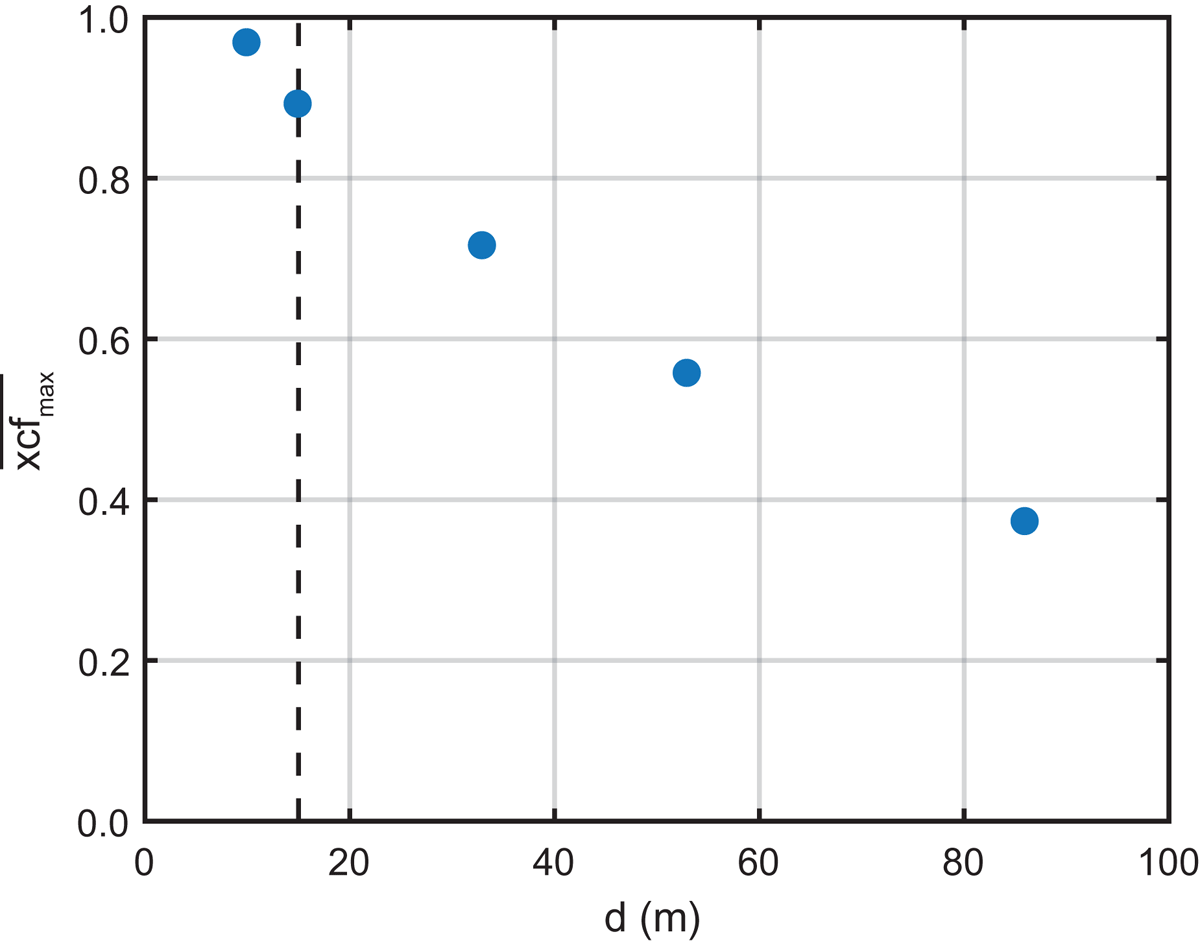
Fig. 4.
Mean maximum cross-correlation () between the air pressure fluctuations of two pressure sensors as a function of distance d. The dashed line indicates the distance d = 15 m.
It is clear that strongly decreases with increasing d. Only for d < 15 m, > 0.90, corresponding to R 2 = 0.81. This demonstrates that the same air pressure fluctuations were measured within a distance of 15 m. At d > 15 m, the differences between the air pressure fluctuations increased significantly. This increase is attributed to amplitude changes and frequency shifts between the two air pressure signals.
Spatial variability of PPC
3.4.
Although the differences between air pressure fluctuations strongly increase when d > 15 m, their envelopes stay similar. Thus, it was investigated if the dependence of PPC on varies when d is changed. In Fig. 5 the dependence of PPC on is shown for d = 0, 35 and 90 m.
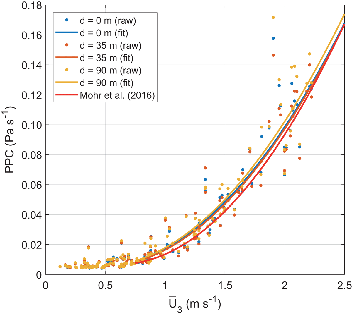
Fig. 5.
Dependence of PPC on mean above-canopy wind speed at height z 3 for the pressure signals at distances d = 0, 35 and 90 m (dots). In addition, the raw data are fitted with a quadratic function (solid lines). The dependence found by Mohr et al. (2016) is shown in red.
Following Mohr et al. (2016), quadratic fits were calculated for the description of the dependences of PPC on for the different distances:
The average error between and is 3.2% and the average error between and equals 3.0%. Therefore, it can be concluded, that PPC calculated from a single air pressure measurement is at least representative for an area within a radius of 90 m.
The average difference between the quadratic fit reported by Mohr et al. (2016) and is 13.0%. This difference might be attributed to the significant difference (Kruskal–Wallis-Test, 1% significance level) in the wind speed distribution observed by Mohr et al. (2016) and observed in this study.
Conclusions
4.
For the first time, the direction and the speed of propagation of air pressure fluctuations responsible for pressure pumping above a forest floor were identified. The air pressure fluctuations propagate in the same direction as the above-canopy airflow and not in the direction of below-canopy airflow. Moreover, the mean propagation speed of the air pressure fluctuations is in the same order as the mean above-canopy wind speed (up to 6.5 m s−1) and increases with increasing mean above-canopy wind speed. These findings indicate that above-canopy airflow is linked to below-canopy air pressure fluctuations that influence soil gas transport through pressure-pumping.
Within a radius of 15 m the same strong peaks of the air pressure fluctuations were observed, but with time lags up to several seconds. The dependence of the pressure pumping coefficient on the mean above-canopy wind speed stays constant within a distance of 90 m.
This result specifies the range of influence of the air pressure fluctuations and helps to assess the number of air pressure measurements needed for the investigation of the influence of pressure pumping on soil gas transport at the measurement site.
Funding
This work has been supported by the German Research Foundation [grant number SCHA 1528/1-1], [grant number SCHI 868/3-1].
Disclosure statement
No potential conflict of interest was reported by the authors.