
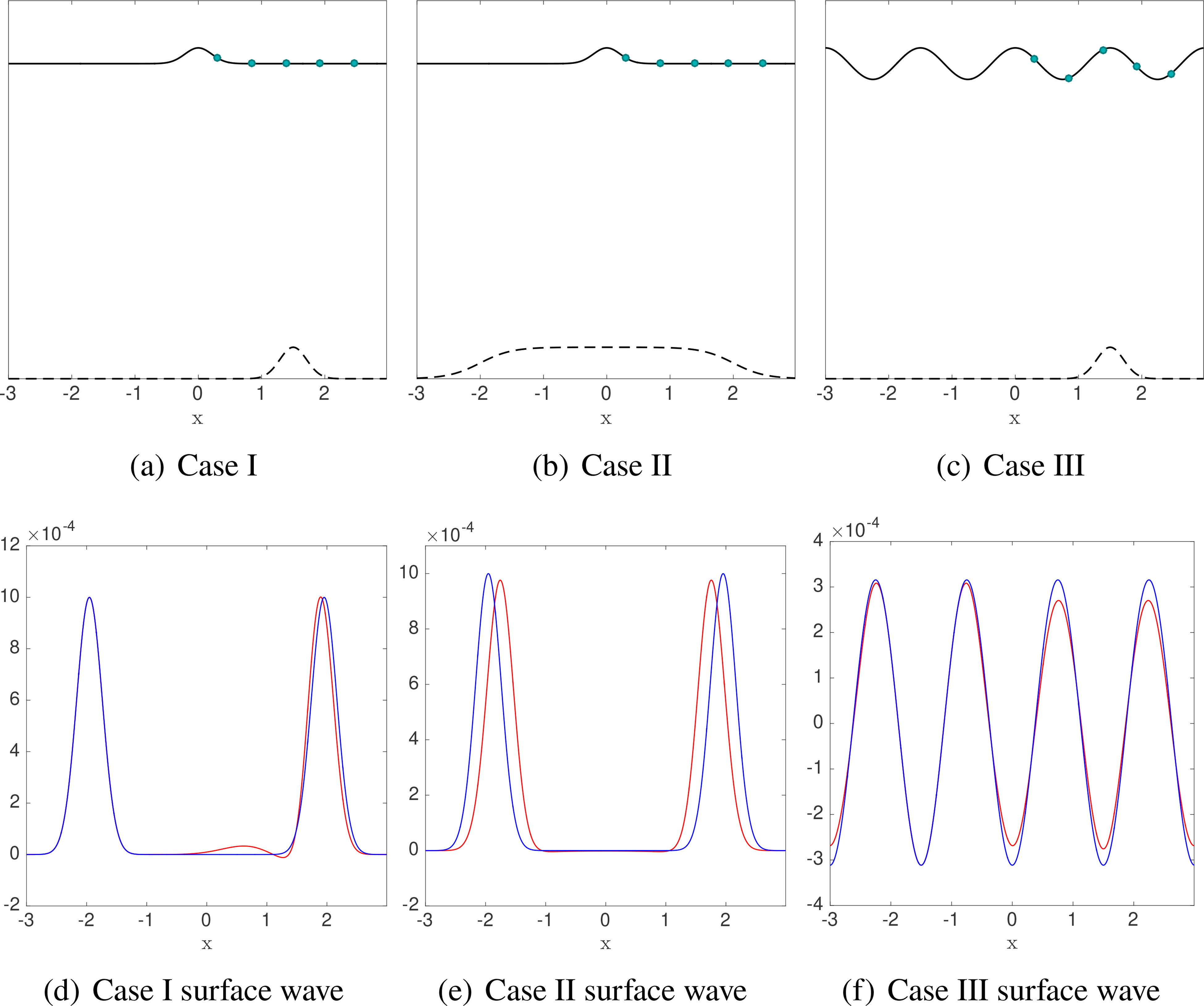
Fig. 1.
(a–c) Three test cases for bathymetry and free surface perturbation initial conditions for the data assimilation scheme. The green circles represent the locations of the observations, with Nobs = 5 and Note that while the spatial distribution is correct, amplitude of the initial conditions amplitude of the bathymetry and average depth H are not to scale in these diagrams, as was restricted to 1% of across most of the numerical tests. Plots (d–f) show the propagating free surface wave at t = 1.95 with flat bottom (blue) and bathymetry (red) for each Cases I, II and III, respectively, to highlight the effect of bathymetry on surface wave propagation.
Table 1.
Notation used in the derivation of data assimilation scheme of the SWE to find the optimal bathymetry, using same format as given in Table 1 of Kevlahan et al. (2019).
Table 2.
Cases considered for data assimilation Algorithm 1.
[i] These bathymetry/initial conditions cases are illustrated in Fig. 1.
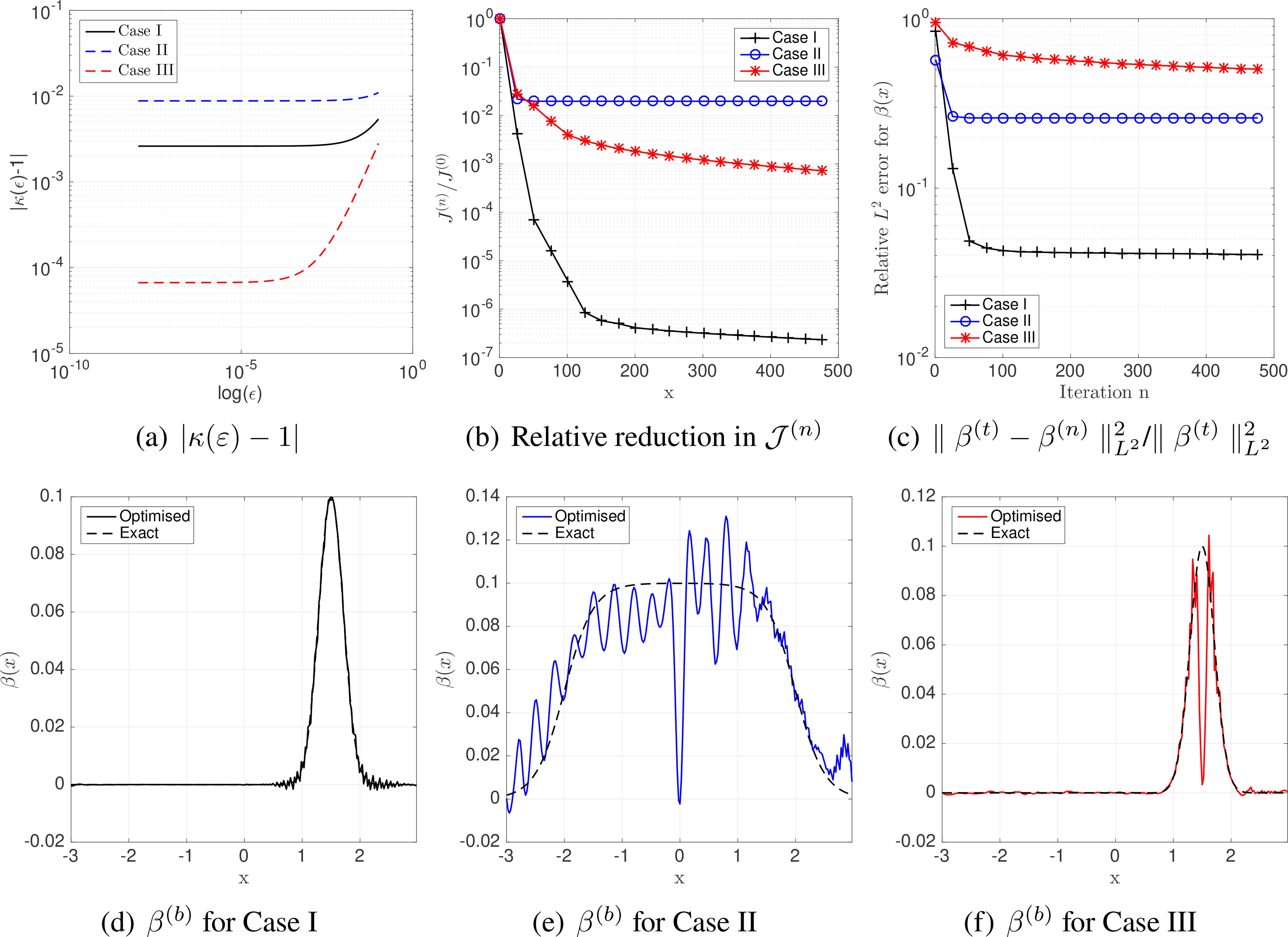
Fig. 2.
Results for iterative data assimilation scheme outlined in Algorithm 1, with Only in Case I do we consider that the assimilation has reconstructed the bathymetry with sufficient accuracy ( relative error). (a) Convergence of the kappa test for the three cases. (b) Relative reduction in the cost function after 500 iterations. (c) Relative error in the reconstructed bathymetry. (d–f) Optimal reconstructed bathymetry for each case. We observe noise in the reconstruction for each case, especially in Case II.
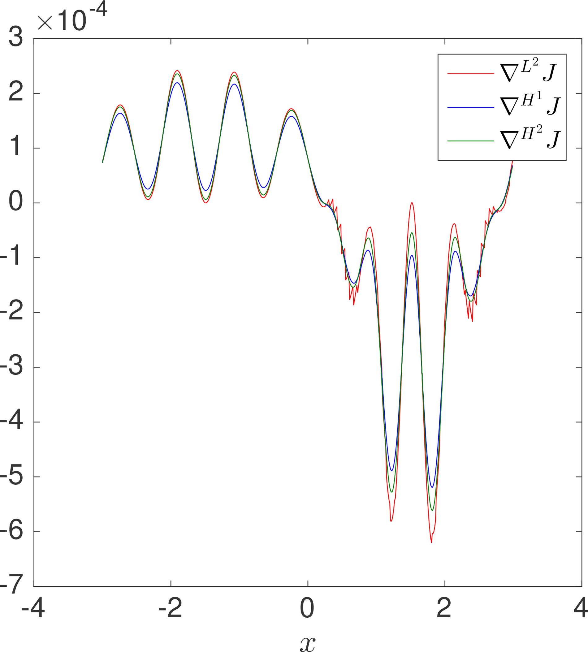
Fig. 3.
The gradient of the cost function obtained after one iteration for Case III, for H 1 and H 2 Sobolev smoothing compared to the (unsmoothed) L 2 gradient.
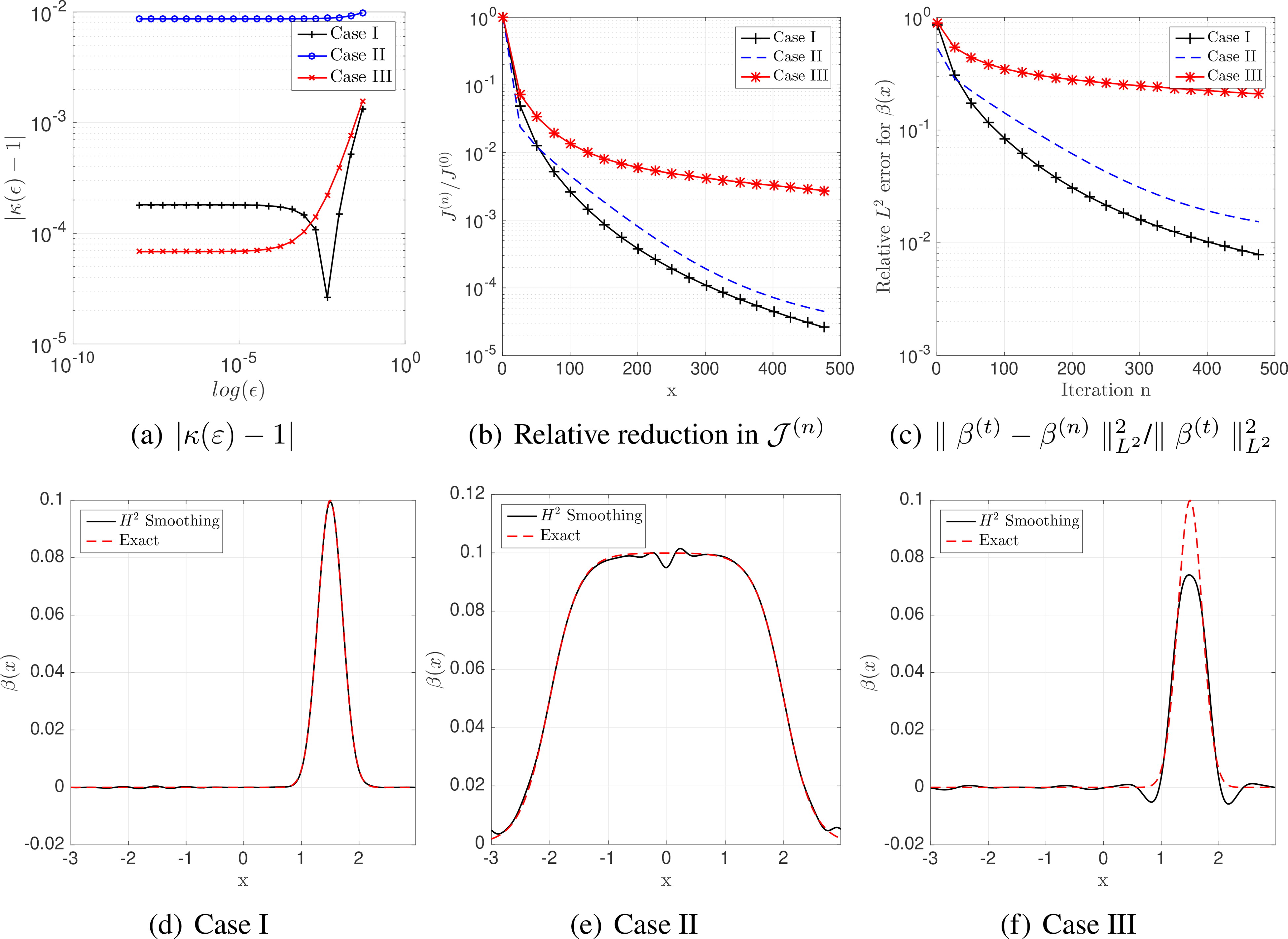
Fig. 4.
Results for assimilation scheme with Sobolev H 2 smoothing applied to (a) Convergence of the kappa test. (b) Convergence of the cost function. (c) Relative L 2 error / between the exact and reconstructed bathymetry at each iteration. (d–f) Reconstructed bathymetry with H 2 smoothing and the exact bathymetry for cases I, II and III, respectively. Convergence is improved compared to results without smoothing given in Fig. 2.
Table 3.
Analysis of six experiments for Case I where and are varying orders of magnitude.
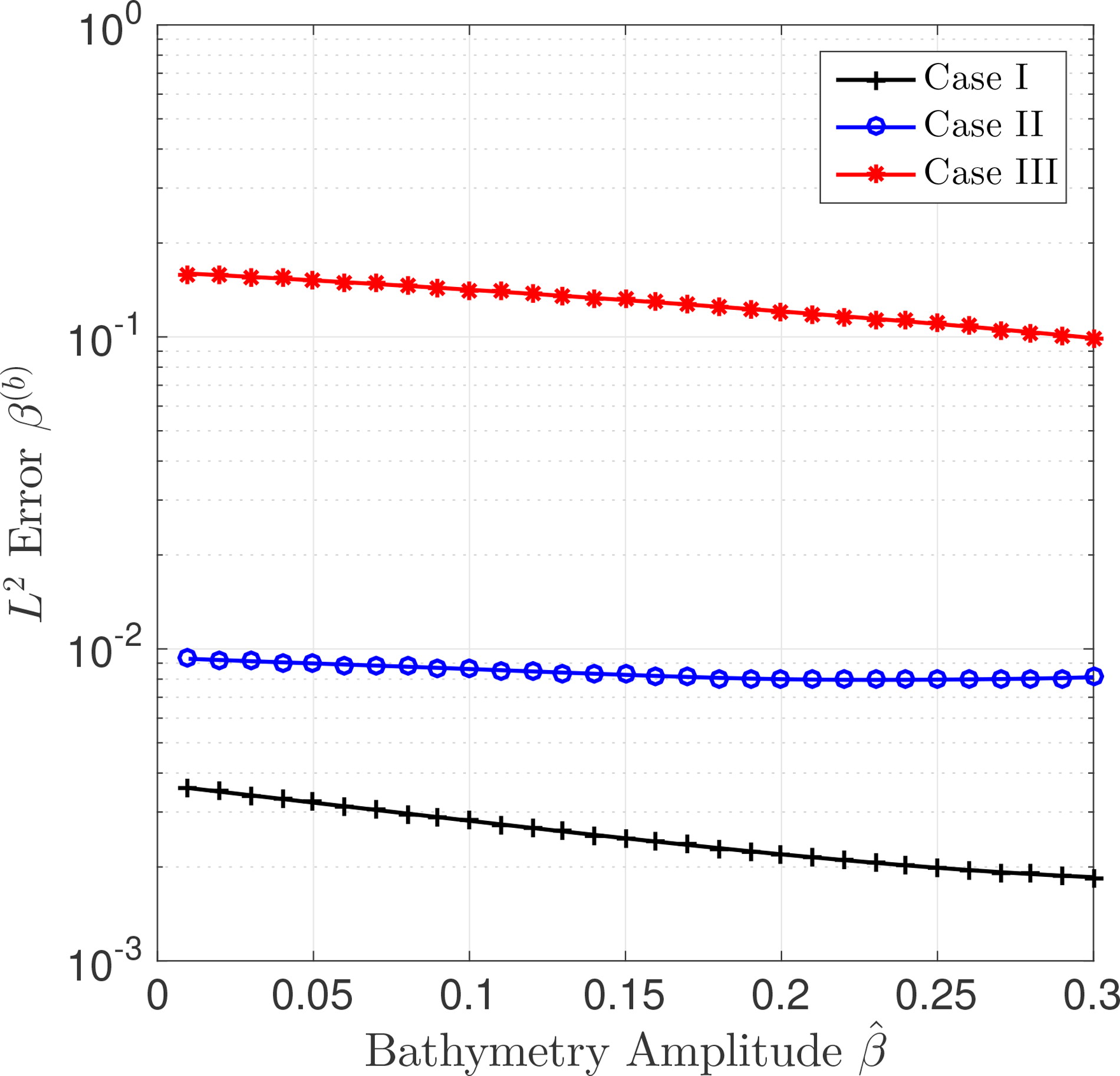
Fig. 5.
The relative error in the bathymetry reconstruction / (where ), shown for different amplitudes with amplitude of initial conditions of H. Note that Case III has barely converged for any value of bathymetry amplitude.
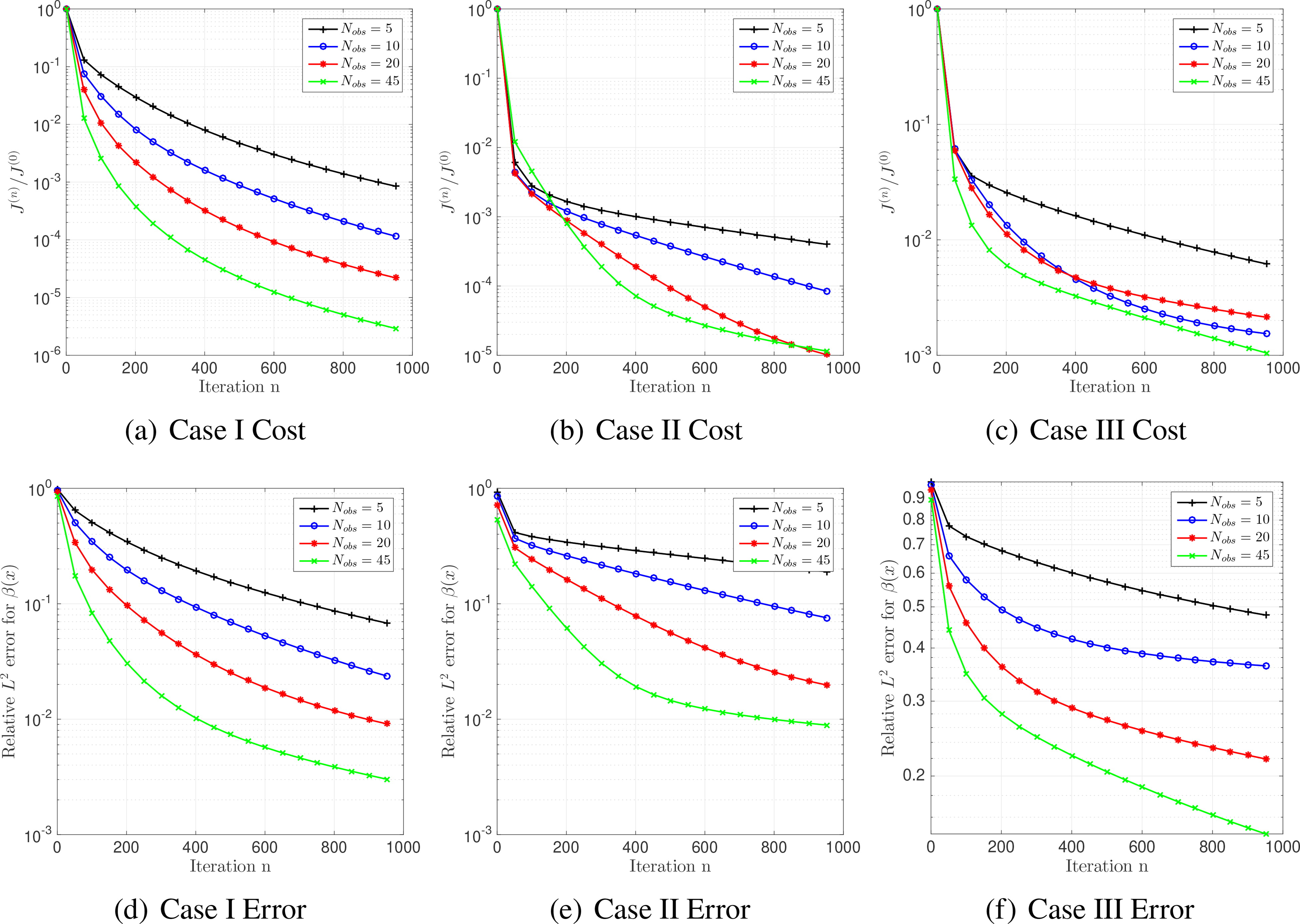
Fig. 6.
Relative cost function and relative L 2 error for different numbers of observation points.
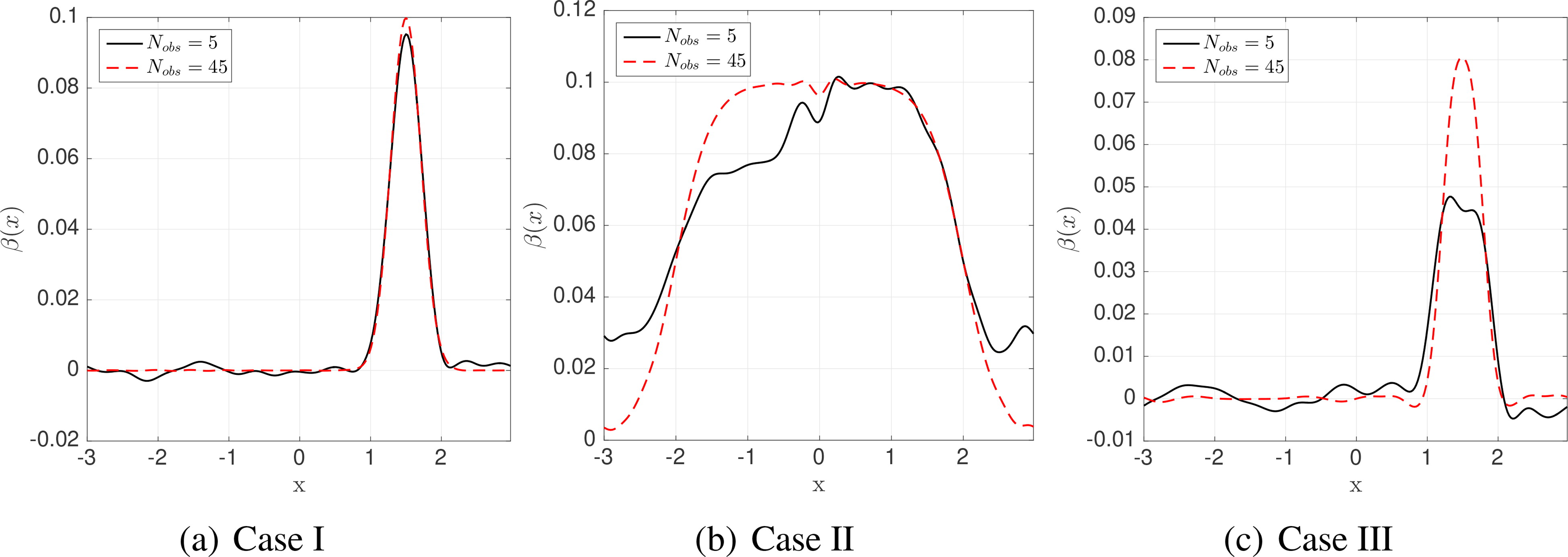
Fig. 7.
Reconstructed bathymetry for Cases I, II and III with Nobs = 5 and Nobs = 45, respectively.
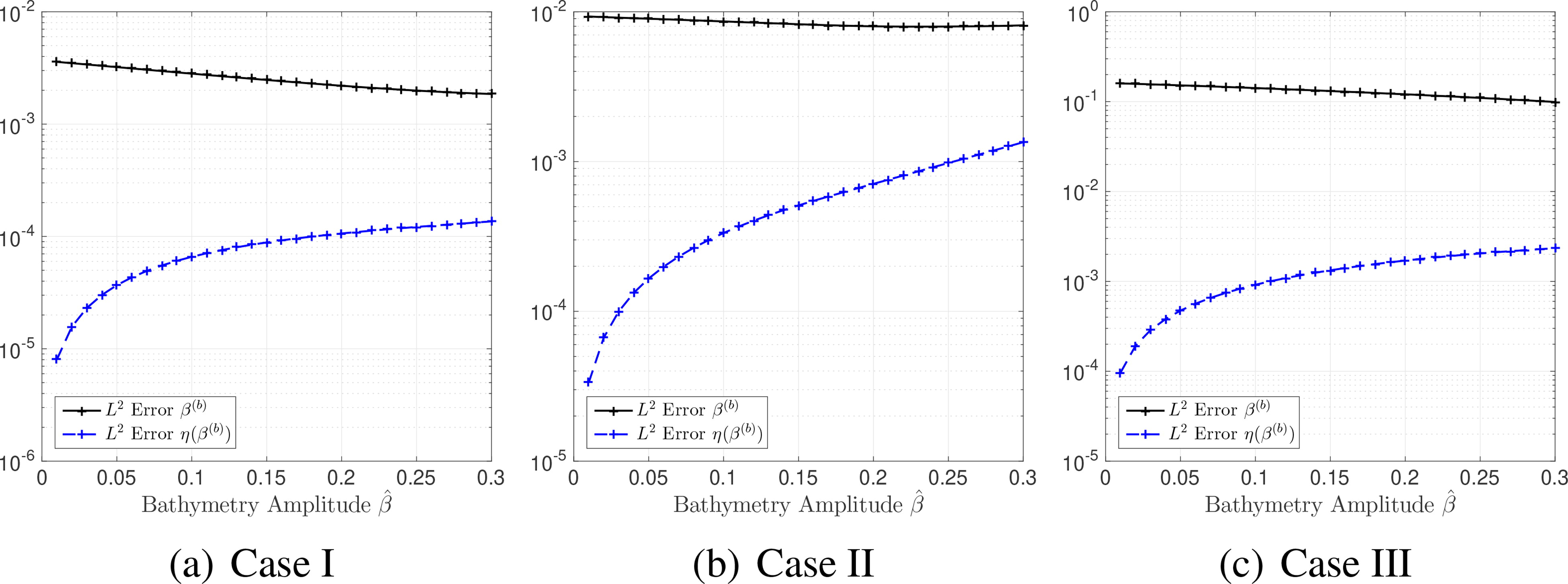
Fig. 8.
The relative L 2 error in the bathymetry reconstruction, shown for different amplitudes and the corresponding relative L 2 error in the propagating surface wave The amplitude of the initial conditions is 0.001, and Nobs = 45.
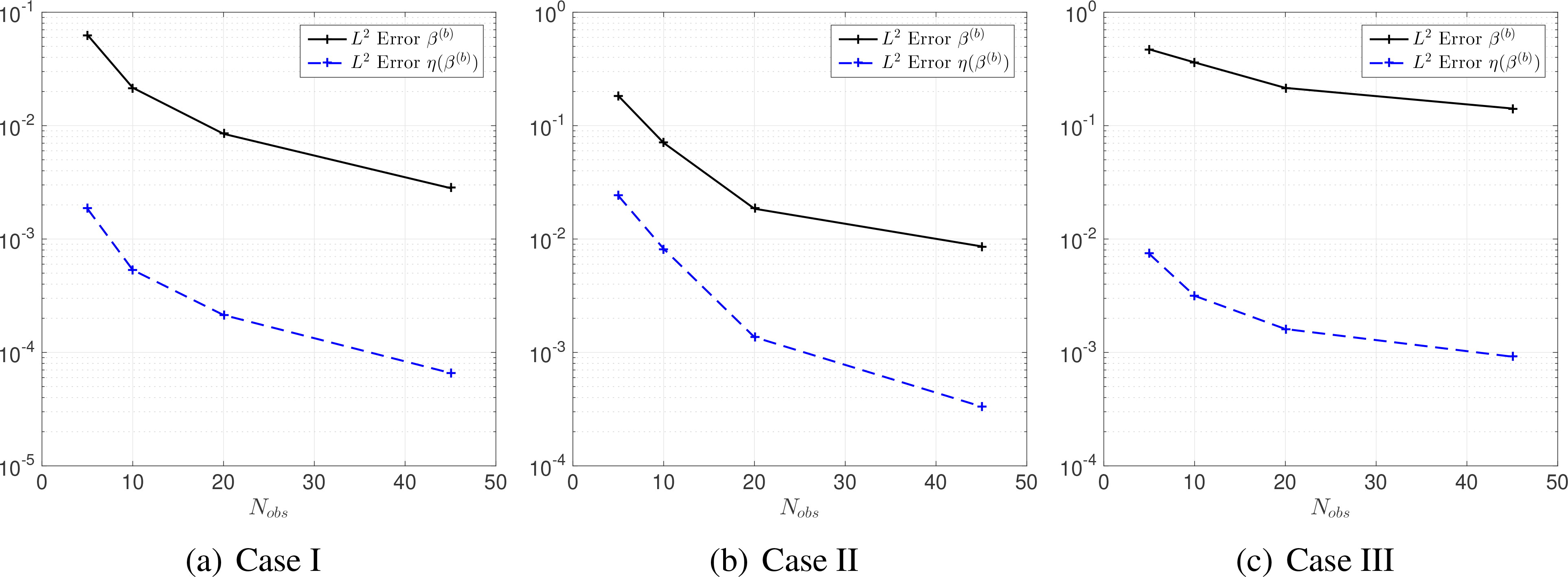
Fig. 9.
The relative L 2 error in the bathymetry reconstruction, shown for different values of Nobs , and the corresponding relative L 2 error in the propagating surface wave The amplitude of bathymetry is 0.1. The amplitude of the initial conditions is fixed to be 1% of
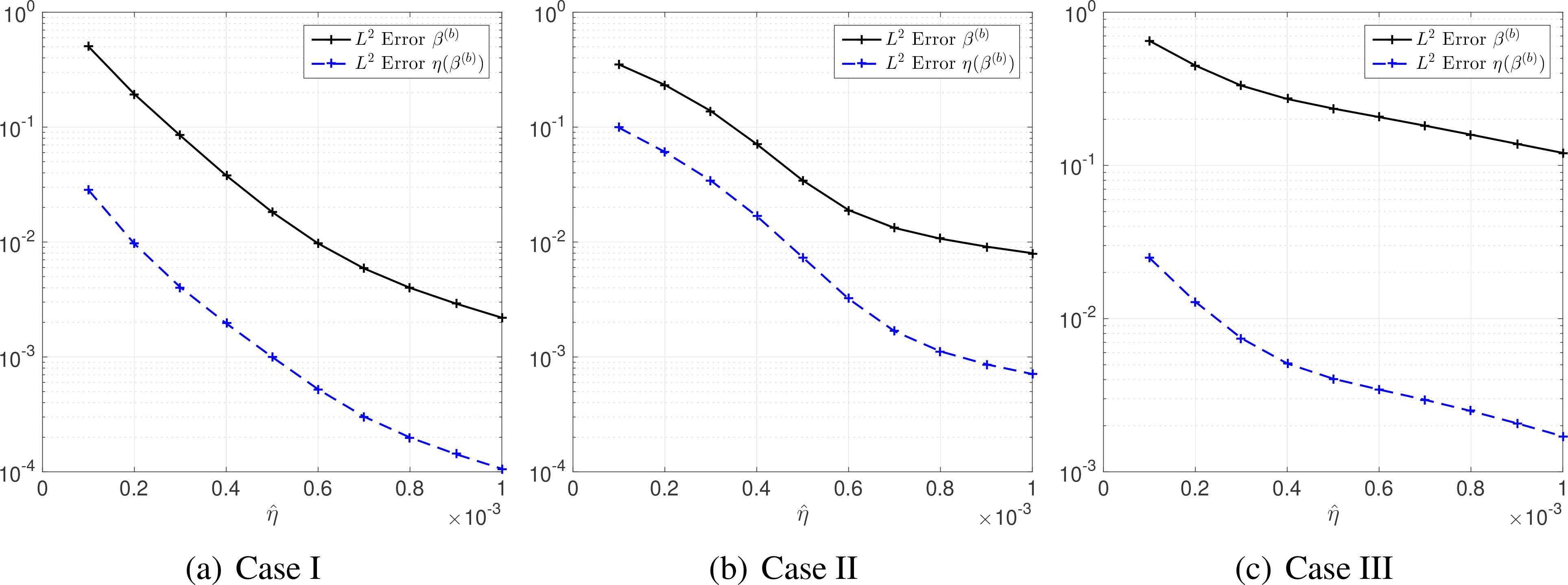
Fig. 10.
The relative L 2 error in the bathymetry reconstruction and the corresponding relative L 2 error in the propagating surface wave as a function of the initial conditions amplitude The amplitude of the bathymetry is fixed to be 0.2.
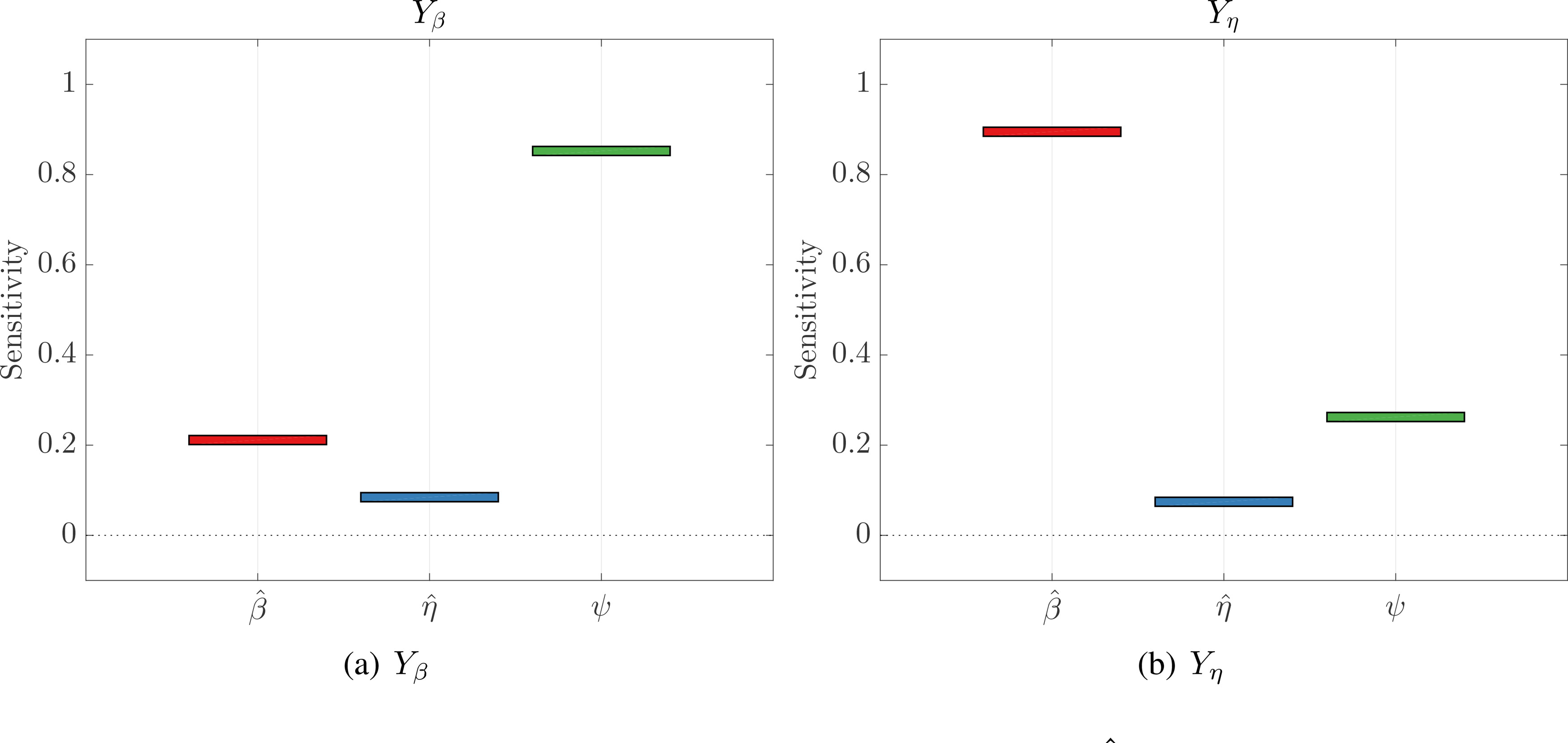
Fig. 11.
Approximation of the density-based sensitivity indices for (red), (blue) and ψ (green). (a) Influence of each parameter on (b) Influence of each parameter on
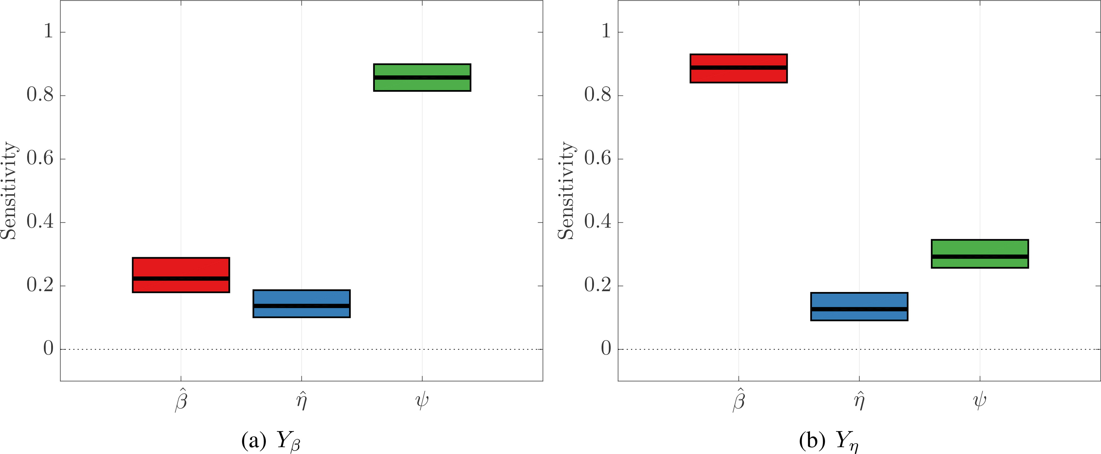
Fig. 12.
Approximation of the density-based sensitivity indices for (blue) and ψ (green), with confidence intervals derived using 700 re-samples. (a) Influence of each parameter on (b) Influence of each parameter on
Table 4.
Width of the confidence interval and mean index averaged over 700 bootstrap re-samples.
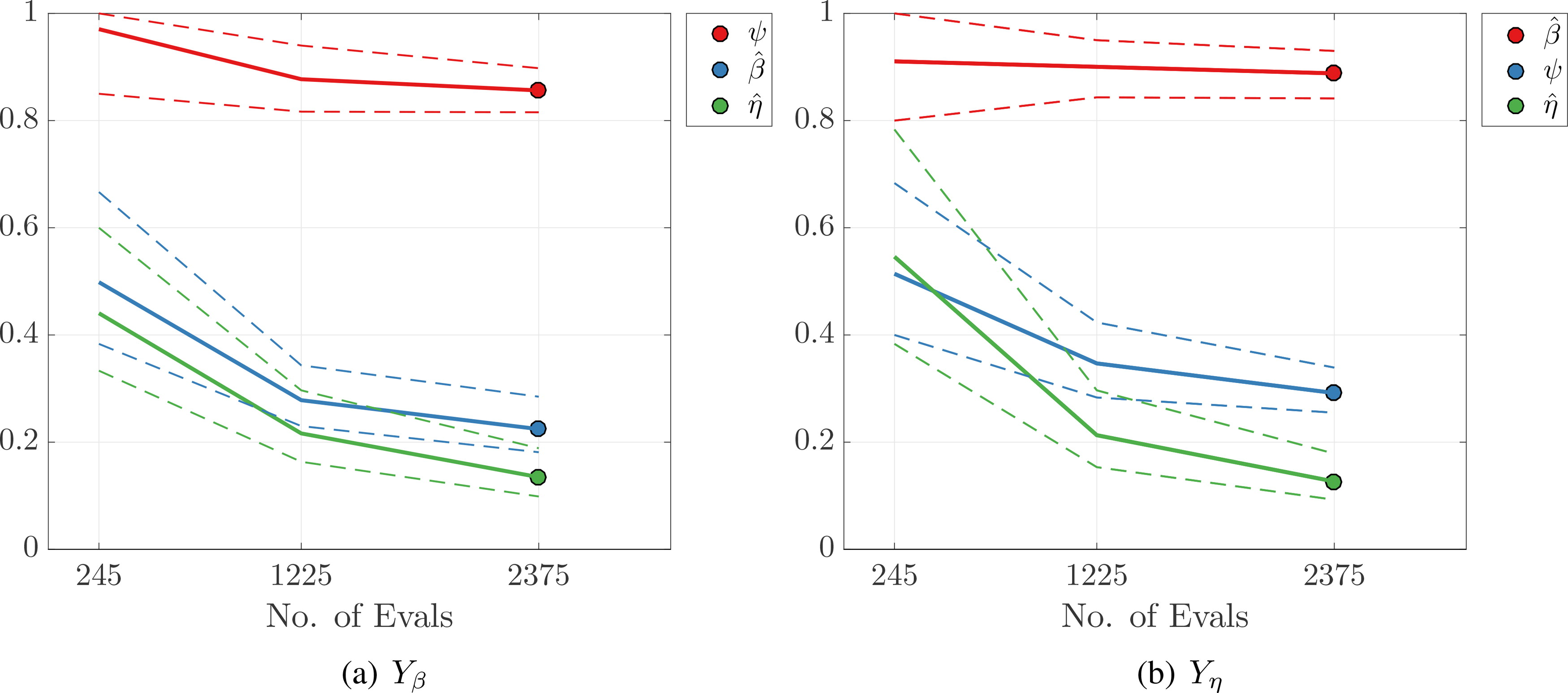
Fig. 13.
Convergence analysis for DBSA indices for (a) and (b) for re-samples of size N = 215 to N = 2375.
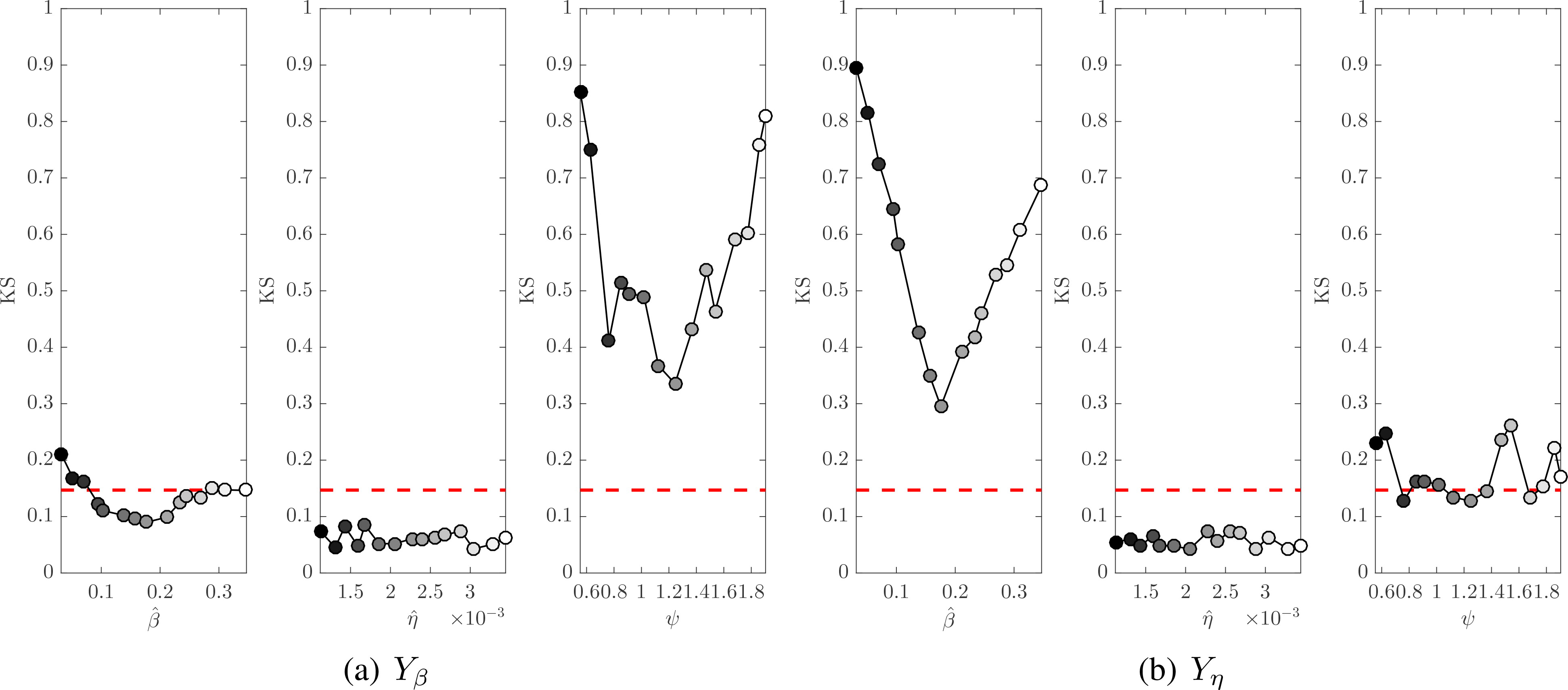
Fig. 14.
KS statistic with significance level 0.05. Values below the dotted red line are non-influential.
Table 5.
Model output indices Ti using different statistics in the definition of the sensitivity index (7.6).
Table 6.
Model output indices Ti using different statistics in the definition of the sensitivity index (7.6).
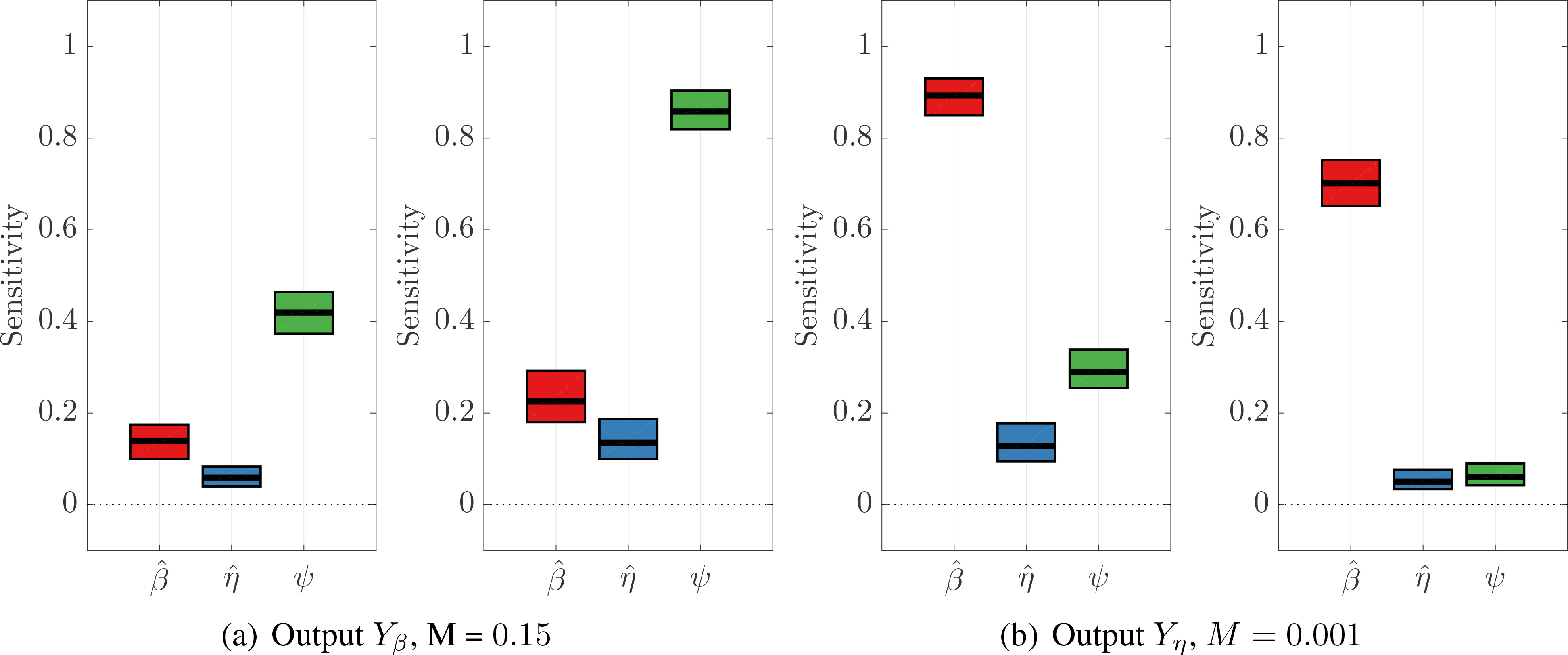
Fig. 15.
Indices Ti for influence of (red), (blue) and ψ (green) on model outputs Y > M (left panel), and (right panel) for (a) and (b) Confidence intervals were calculated using 700 bootstrap samples.
Table 7.
Classification of each input parameter as influential or non-influential for the sub-regions of and in Fig. 15.
[i] Values below the threshold value of 0.147 () are non-influential. The entries highlighted in blue are the most influential parameter for and respectively. is influential on bathymetry reconstruction error only when the error is larger than 0.15, and ψ is only influential on the surface wave error when the error is larger than 0.001.