
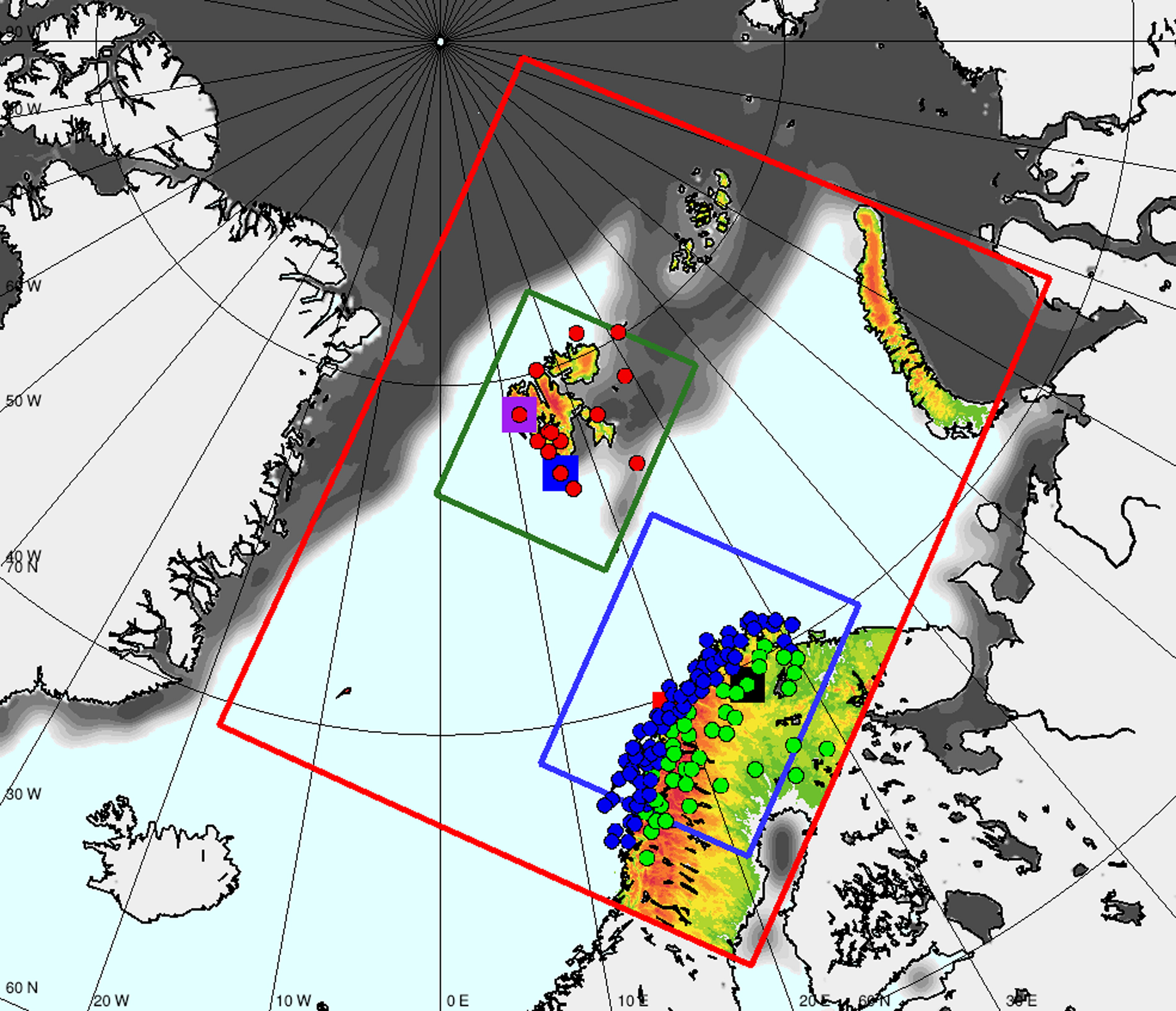
Fig. 1.
Regional integration domains. The operational AROME-Arctic/CNTRL-experiment in red, the Svalbard domain in green and the North Norway domain in blue. The Observation sites used for evaluation; inland (green circles), coast and fjords (blue circles) and Svalbard stations (red circles). In addition, individual observation sites used for time series are marked with colored squares—Hornsund (blue), Ny-Ålesund (purple), Tromsø (red) and Karasjok (black). Orography in CNTRL-experiment shown in white/green (0–100 masl) to red colors (more than 1000 masl). Sea ice concentration (8 March 2018) from the operational IFS-HRES is shown in grey with darker shades indicating higher concentrations.
Table 1.
Summary of experiments.
[i] Configurations unique for the different experiments in bold. Experiments; CNTRL (control experiment), EPS (1 + 10 member), ATMASS (upper-air assimilation), DD (Dynamical Downscaling), HIGHRES (finer horizontal and vertical resolution), SVA (small domain around svalbard) and NN (small domain around Northern Norway). The cost column is relative to the CNTRL experiment (EPS is relative to 1 EPS member). The regional domains are shown in Fig. 1 and large refers to the operational AROME-Arctic domain.
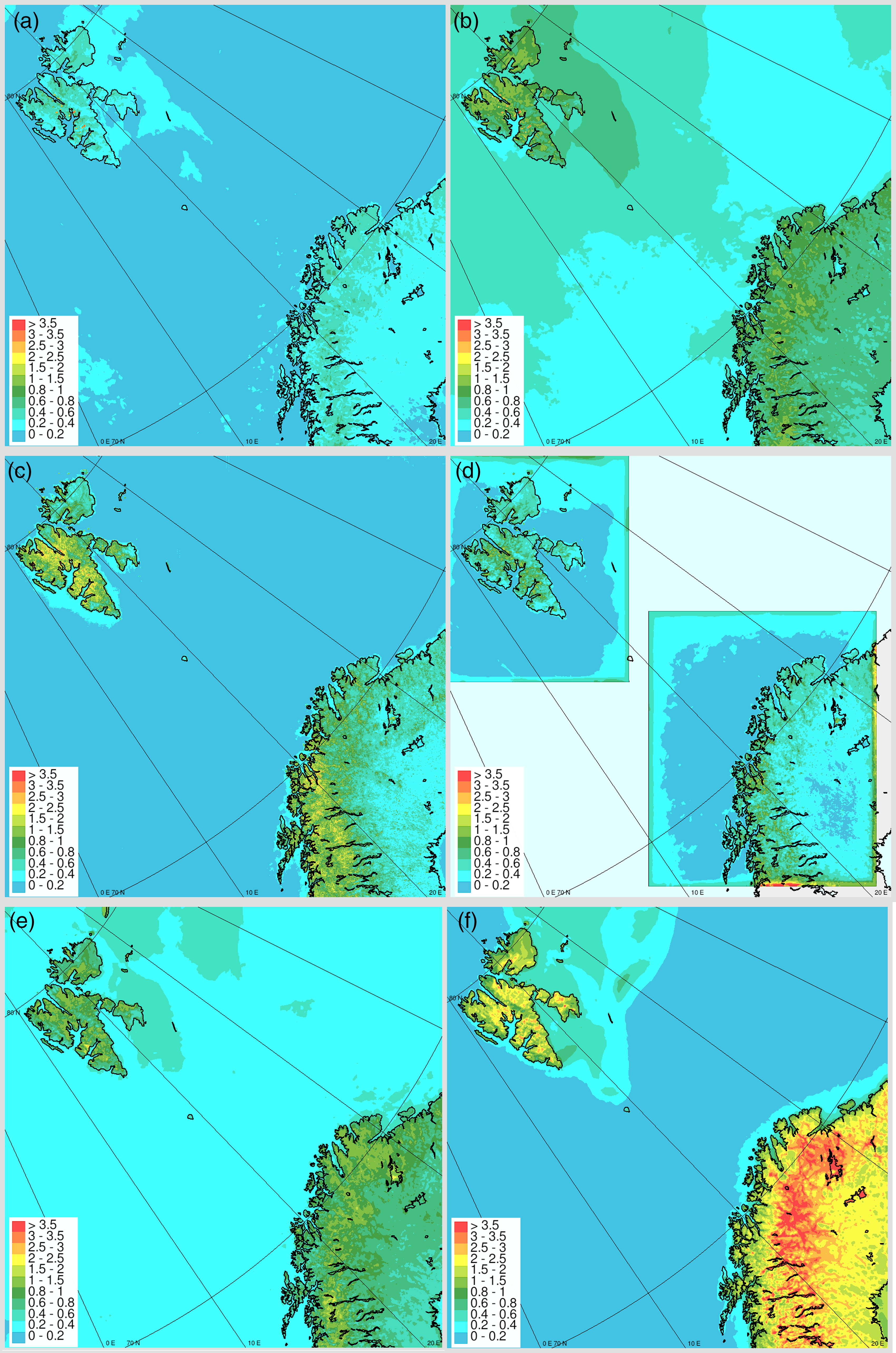
Fig. 2.
Potential Change in Forecast Quality measured by Mean Absolute Difference in T2m [°C] averaged over day 1 forecasts 8–31 March 2018 for (a) EPS: EPS mean vs. EPS control member, (c) higher spatial resolution: HIGHRES vs. CNTRL, (d) domain size/location: SVA/NN domains vs. CNTRL, (e) initialization atmosphere: ATMASS vs. CNTRL and (f) Initialization surface: CNTRL vs. DD. In addition, (b) predicting the forecast uncertainty: the average ensemble spread [°C].
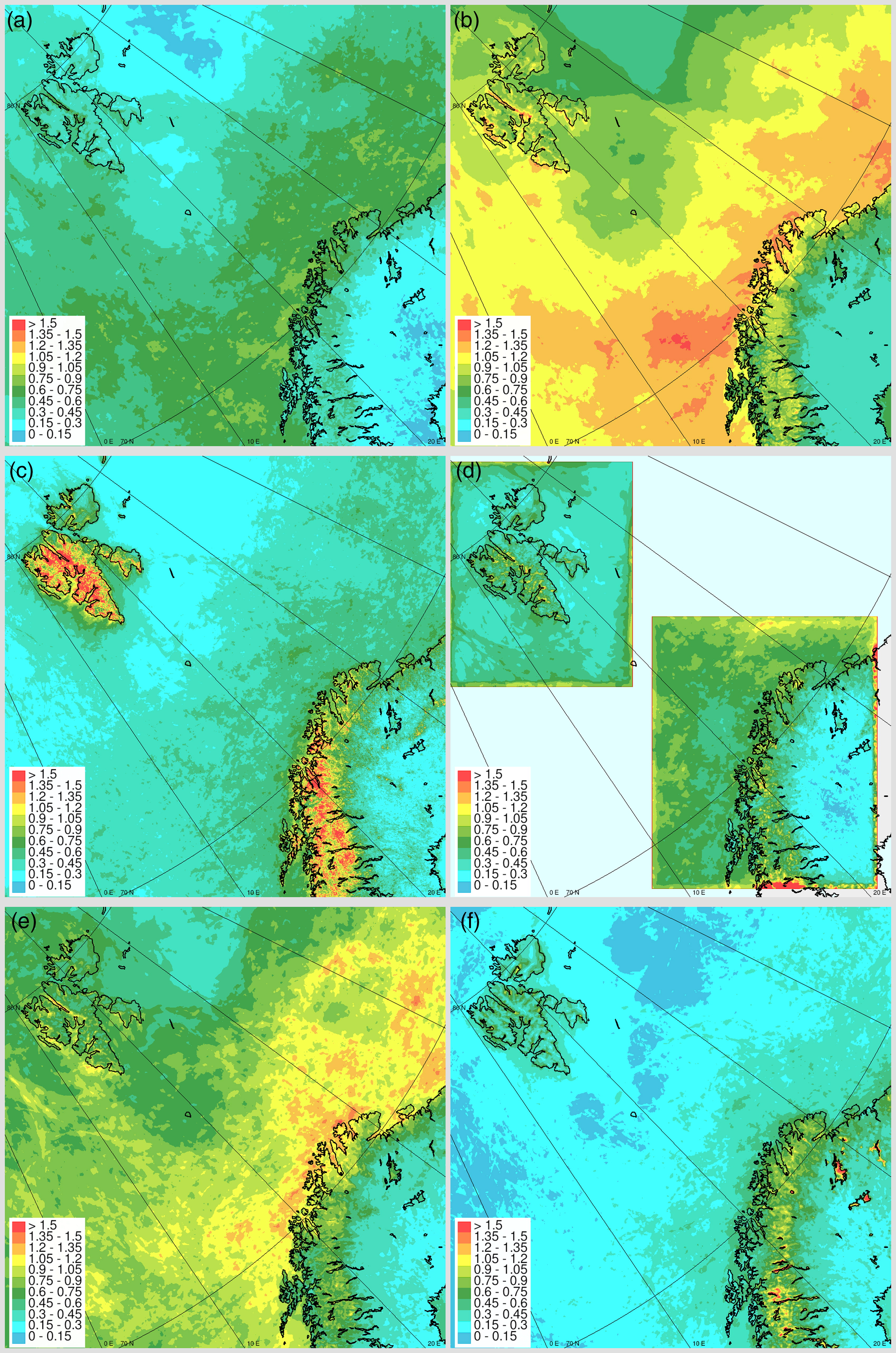
Fig. 3.
As Fig. 2, but for 10 m wind speed, WS10 [m/s].
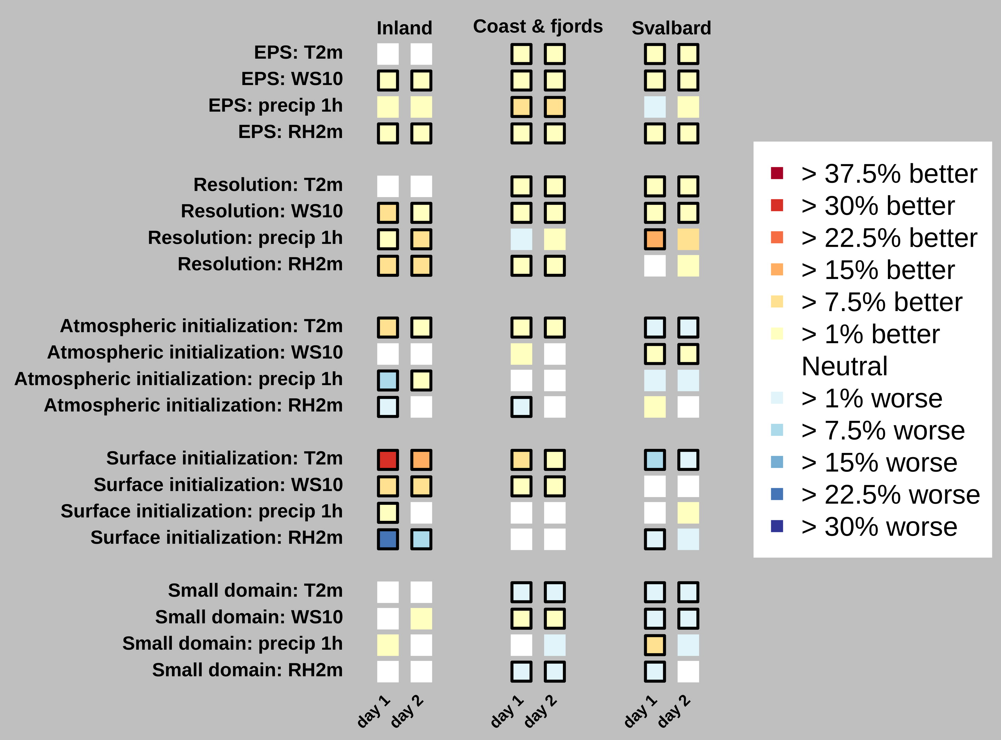
Fig. 4.
Changes in forecast quality by EPS (EPS mean vs. EPS control member), higher spatial Resolution (HIGHRES vs. CNTRL), atmospheric initialization (ATMASS vs. CNTRL), surface initialization (CNTRL vs. DD) and using small domains (SVA/NN vs. CNTRL) measured by mean absolute error skill score for day 1 and day 2 forecasts. Parameters are T2m, WS10, precip and RH2m. Black frames indicate a significant difference in the verification score at the 95%-level calculated by bootstrapping.
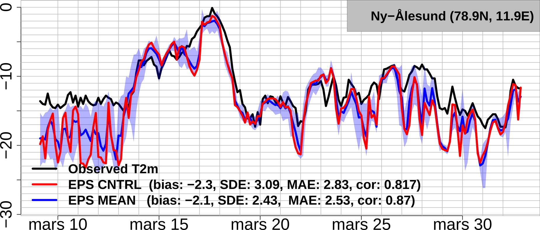
Fig. 5.
Time series of T2m at Ny-Ålesund, observations (black), ensemble mean (blue), ensemble maximum/minimum (blue shading) and the non-perturbed control member (red). Forecasts are initialized at 00 UTC and lead times +27, +30, +33, +36, +39, +42, +45 and +48 h are used.
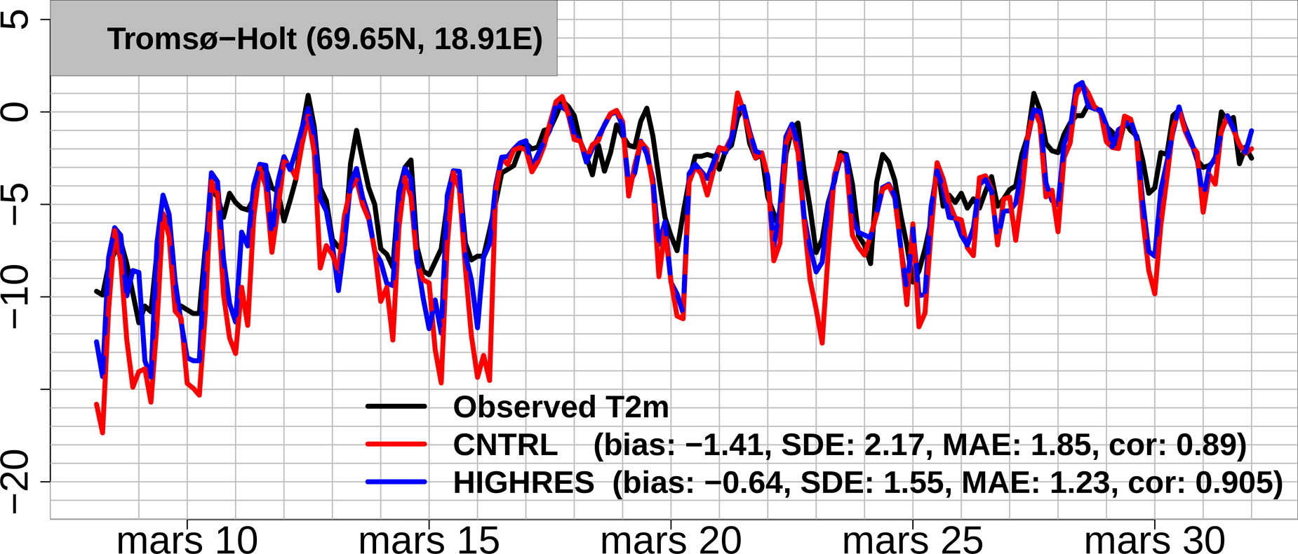
Fig. 6.
Time series of T2m at Tromsø-Holt, observations (black), HIGHRES (blue) and CNTRL (red). Forecasts are initialized at 00 UTC and lead times +3, +6, +9, +12, +15, +18, +21 and +24 h are used.
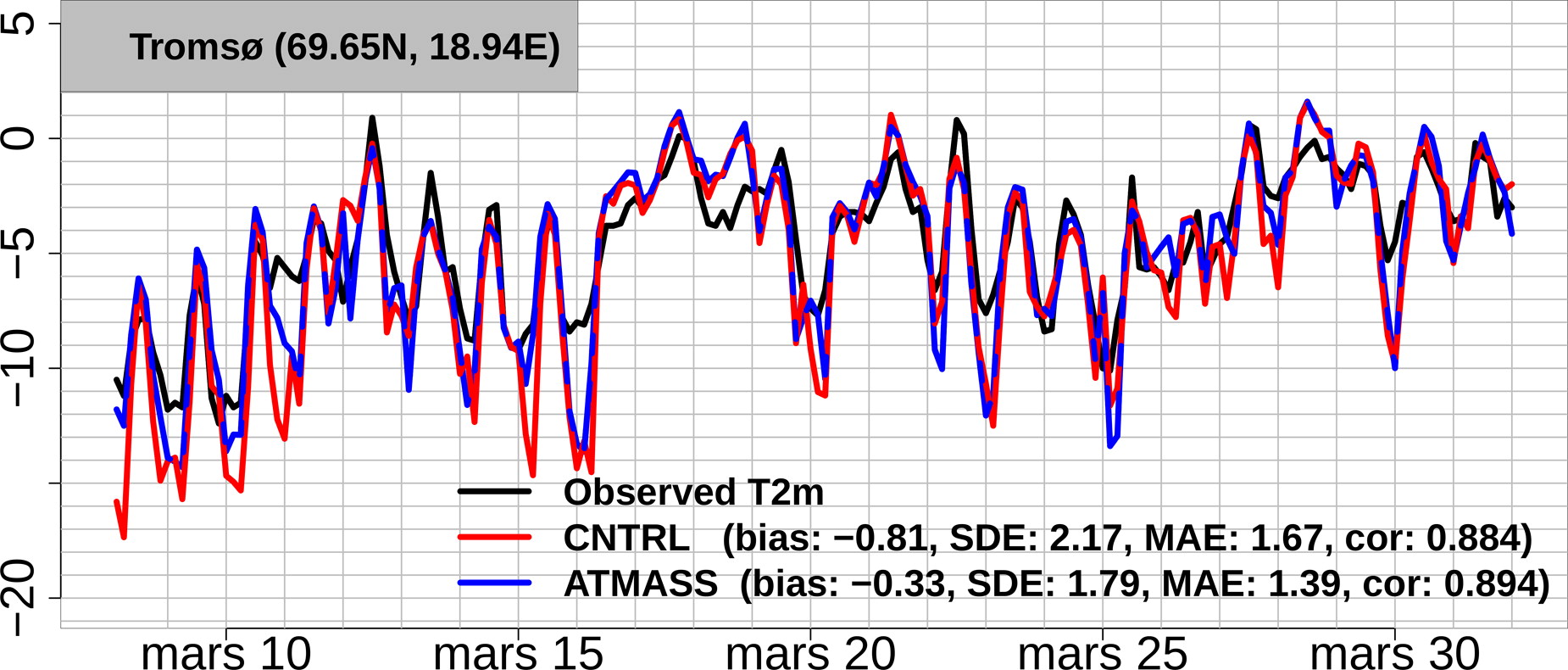
Fig. 7.
Time series of T2m at Tromsø (close to Tromsø-Holt in Fig. 6), observations (black), ATMASS (blue) and CNTRL (red). Forecasts are initialized at 00 UTC and lead times +3, +6, +9, +12, +15, +18, +21 and +24 h are used.
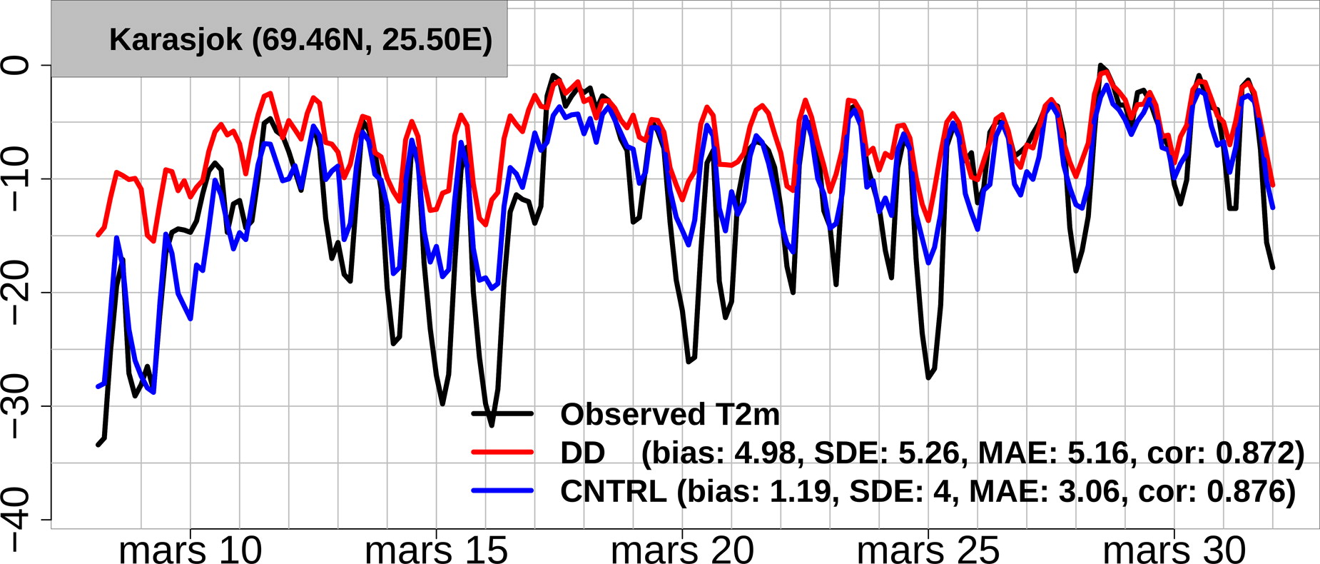
Fig. 8.
Time series of T2m at Karasjok, observations (black), CNTRL (blue) and DD (red). Forecasts are initialized at 00 UTC and lead times +3, +6, +9, +12, +15, +18, +21 and +24 h are used.
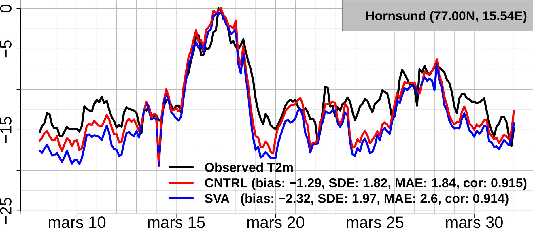
Fig. 9.
Time series of T2m at Hornsund, observations (black), small domain (blue) and CNTRL (red). Forecasts are initialized at 00 UTC and lead times +3, +6, +9, +12, +15, +18, +21 and +24 h are used.
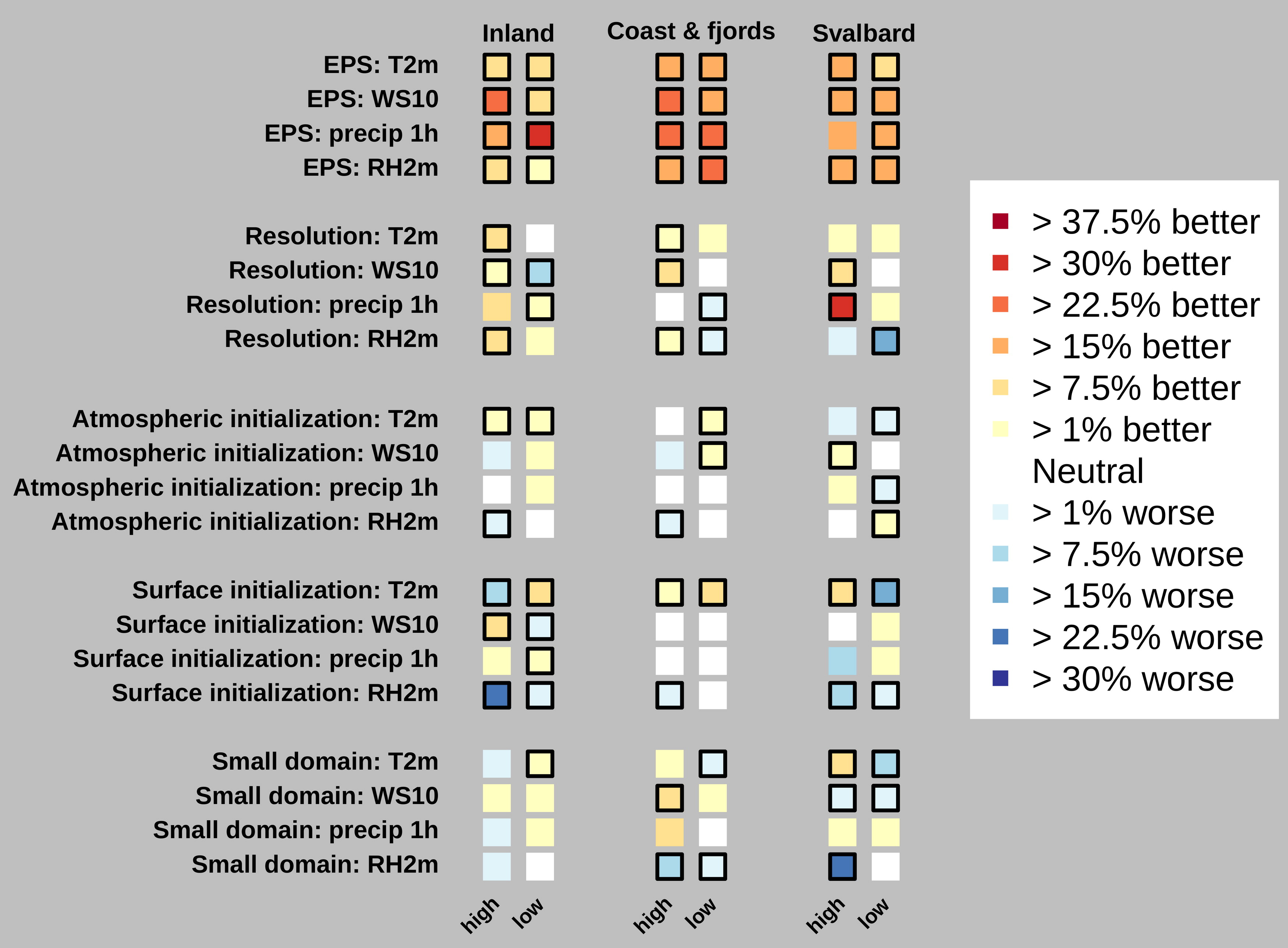
Fig. 10.
Changes in forecast quality of tail events by EPS (EPS mean vs. EPS control member), higher spatial Resolution (HIGHRES vs. CNTRL), atmospheric initialization (ATMASS vs. CNTRL), surface initialization (CNTRL vs. DD) and using small domains (SVA/NN vs. CNTRL) measured by Brier Skill Score for observed low and high tail events. Parameters are T2m, WS10, precip and RH2m. Black frames indicate a significant difference in the verification score at the 95%-level calculated by bootstrapping.
Table 2.
Absolute values of thresholds used to define observed tail events during the period 8–31.March 2018.
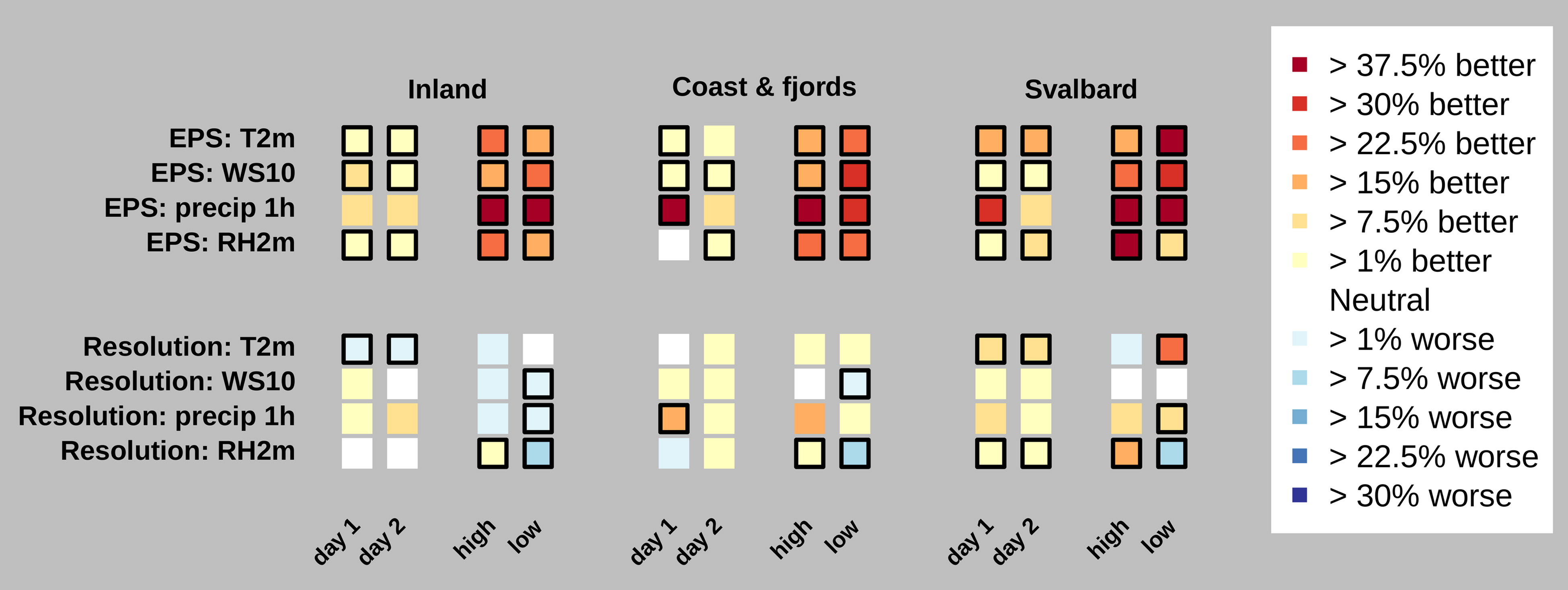
Fig. 11.
Summer period (10 July–1 August, 2018), change in MAE for day 1 and day 2 forecasts and Brier Score for high and low tail events. Similar to what is shown in Figs. 4 and 10, respectively.
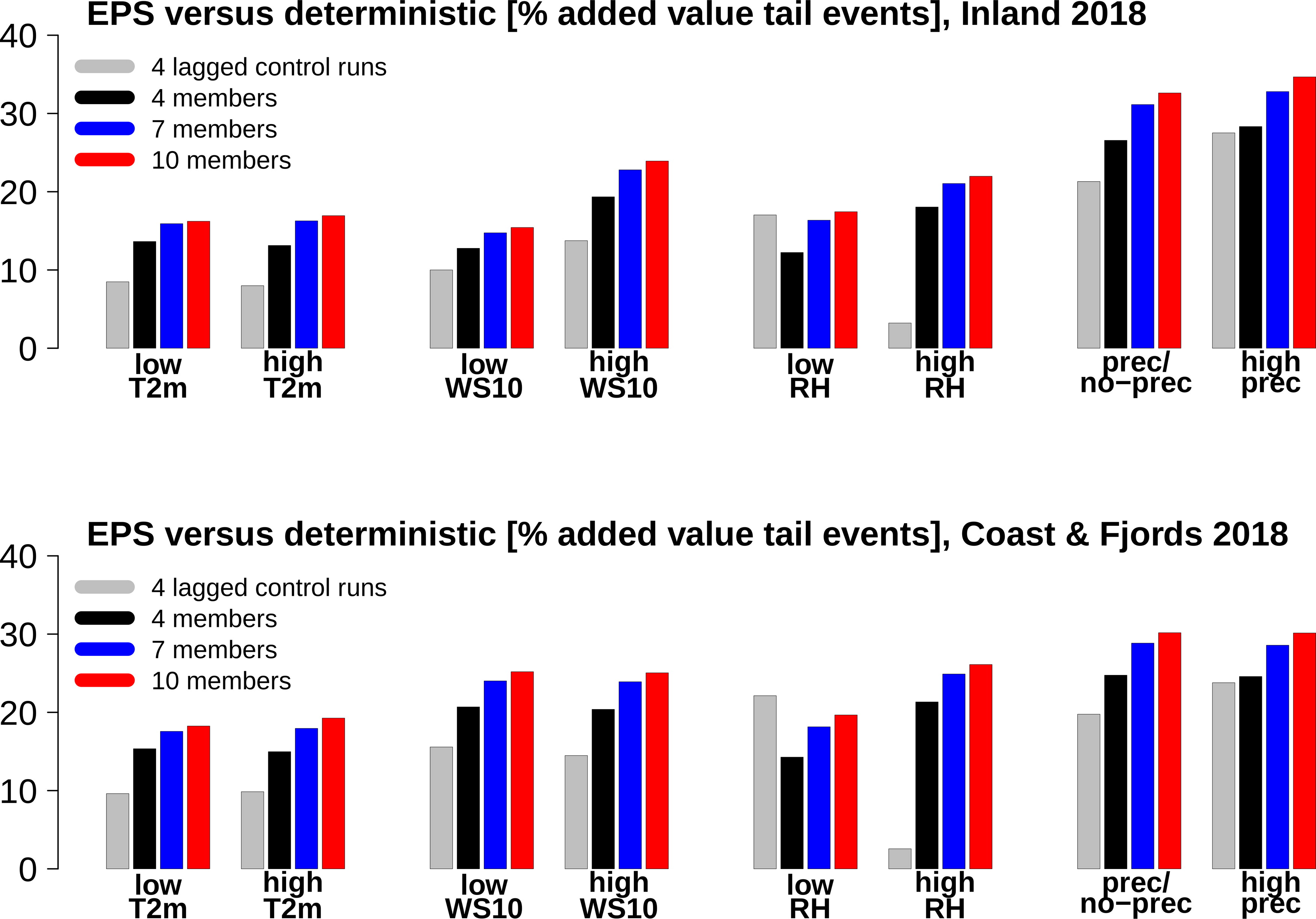
Fig. 12.
Added value measured by Brier Skill Score for low/high tail events, defined for each month similar as in Fig. 10, and then averaged over all months, for inland (top) and coast and fjord (bottom) stations averaged over 2018.