
Table 1.
Important parameters for KENDA COSMO-HH.
Table 2.
Estimated standard deviations of observation errors for assimilated variables.
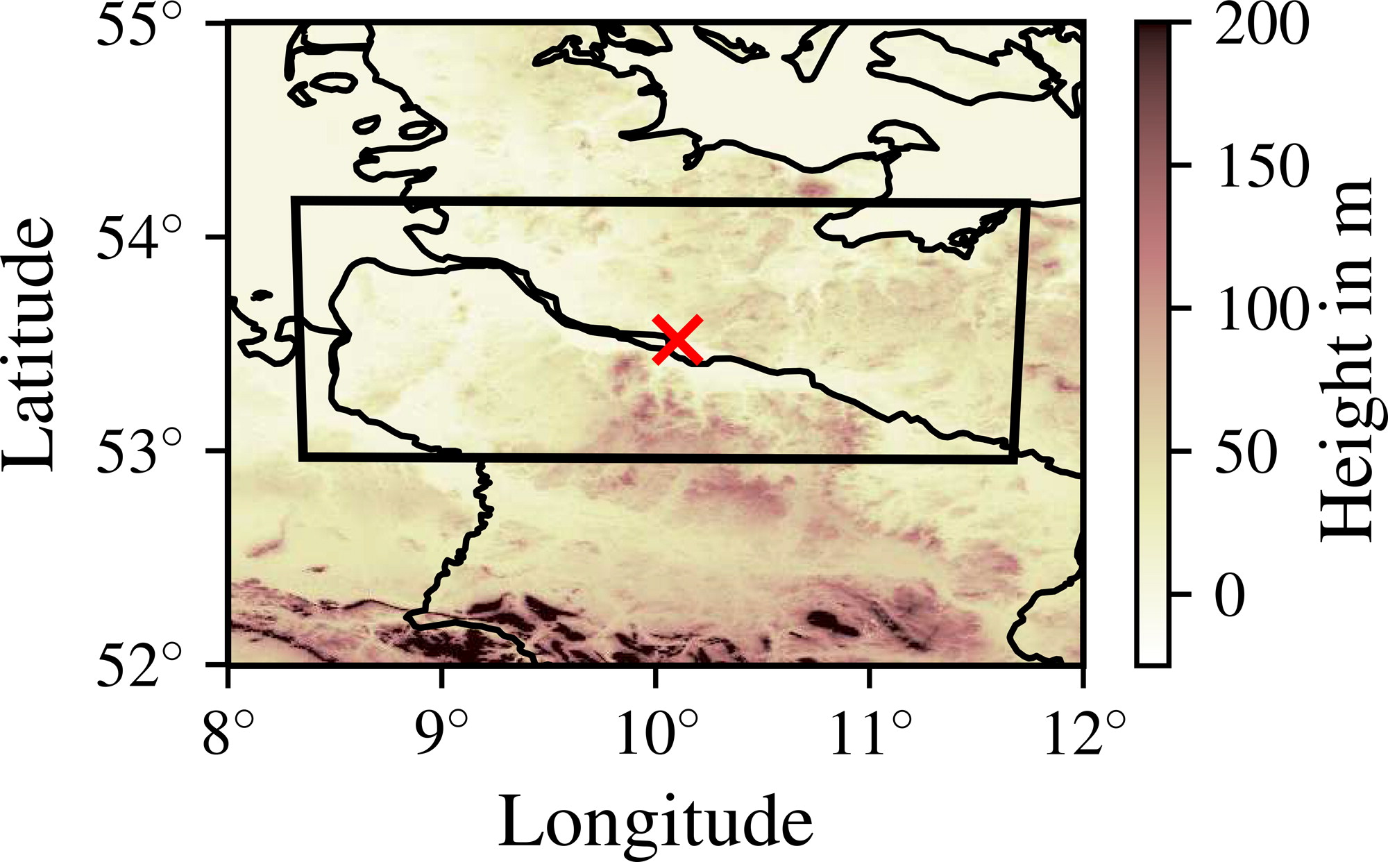
Fig. 1.
Surface height in meters for the metropolitan area of Hamburg. The black rectangle is showing used model area, and the red cross is marking the position of the Wettermast Hamburg. Data are based on NASA JPL (2013).

Fig. 2.
Wettermast levels (except 2-m height) and main model levels for COSMO-HH in the lowest 600 m.
Table 3.
The used measurements at the Wettermast Hamburg with measurement instrument, heights and instrumental accuracy.
Table 4.
Experiment names and assimilated variables.

Fig. 3.
Normalized increment for different variables in (a) & (b) the WIND experiment and (c) & (d) the ALL experiment. (a) & (c) represent the mean absolute increment, while (b) & (d) are the mean increment. Different coloured bars show an observation impact on different variables. Shown increments are normalized by their observation errors. Values are calculated based on ensemble mean of analysis and background for all analysis times and all heights starting in 10 meters at the Wettermast Hamburg. The black lines represent the bootstrapped 5% and 95% percentile based on 1000 samples.
Table 5.
Mean error between ensemble mean in CONTROL experiment and Wettermast Hamburg for U- and V-wind component, temperature, relative humidity, wind speed and stratification. The mean error is estimated over all three test cases and all heights, starting in 10 meters at the Wettermast Hamburg.

Fig. 4.
Mean absolute increment of wind speed (top) and temperature (bottom) for WIND (left) and ALL experiment (right) at the second lowest model level (∼35 m above ground). The spatial average is shown as additional information, while position of the Wettermast Hamburg is marked by a black cross. Land-sea and German state borders are displayed as dark grey contour lines (based on GeoBasis – DE/BKG 2018). (a) Mean = 0.59 m/s, (b) mean = 0.72 m/s, (c) mean = 0.40 K and (d) mean = 0.45 K.
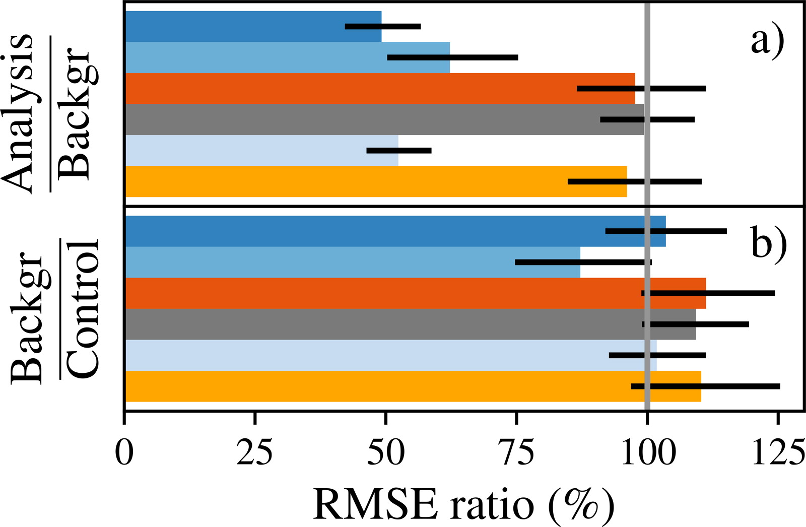
Fig. 5.
Quotient of RMSE between ensemble mean in analysis and in background forecast (a) and quotient of RMSE between ensemble mean in background forecast and for CONTROL experiment (b). Ratios are valid for WIND experiment and are averaged over all analysis times and all heights, expect 2-meter height. Coloured bars have the same meaning as in Figure 3. The black lines represent the bootstrapped 5% and 95% percentile based on 1000 samples.
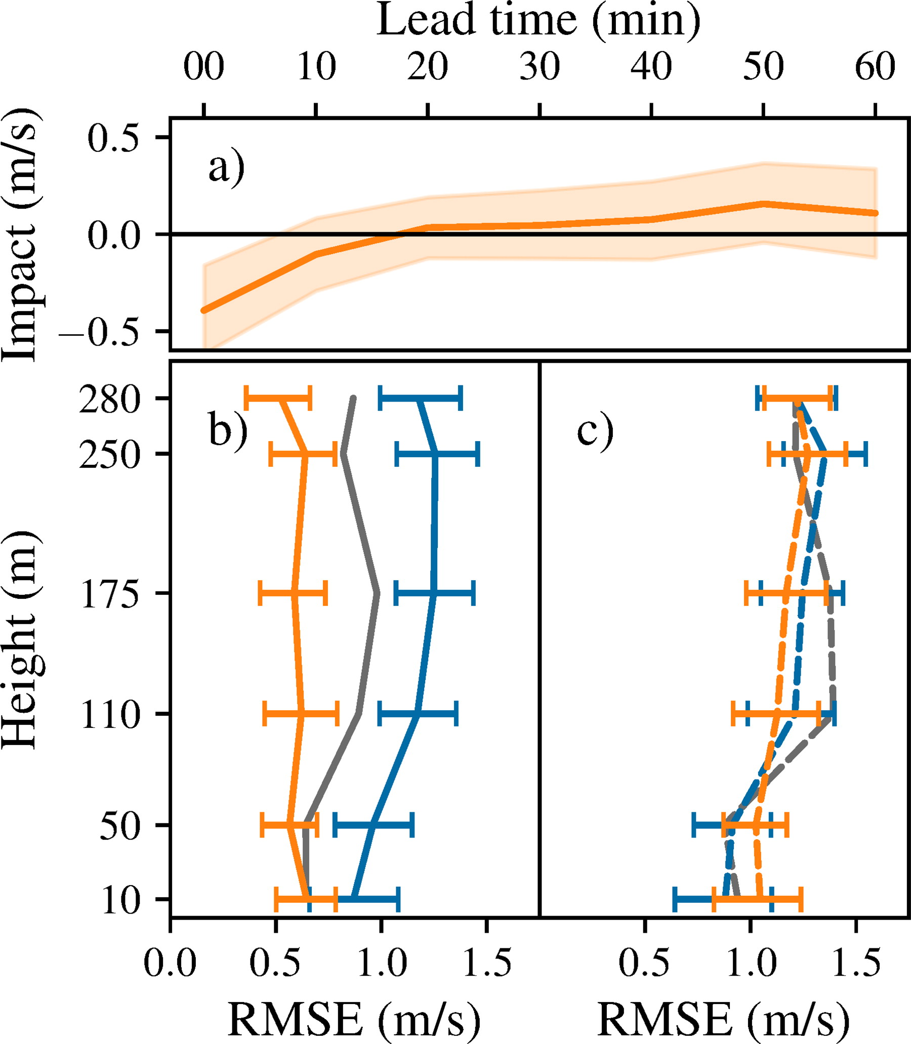
Fig. 6.
The assimilation impact (a), defined as RMSE difference between WIND and CONTROL, for wind speed in 50-m height. Root-mean-squared error of wind speed for (b) analysis (solid lines, left) and for (c) forecasts with one-hour lead time (dashed line, right) against observations as function of height and based on all run times. Three experiments are shown as different colours (Orange: WIND experiment; Grey: ALL experiment). The values for the blue CONTROL experiment are almost the same in (b) and (c), the differences are caused by the time shift of one hour. Displayed error bars and the tube are calculated based on bootstrapping with 1000 samples and represent the 5% and 95% percentile of the RMSE. The error bars for the ALL experiment in (b) and (c) are not shown, because they are almost the same as for the WIND experiment.

Fig. 7.
Time series of wind speed difference between interpolated model output and observations in 50-meter height for all three test cases (a for 07 June 2016, b for 25 October 2016 and c for 12 November 2016). Four different colours show four different types of forecast (Blue: CONTROL experiment without assimilation; Orange: six-hour forecast started with analysis of WIND experiment at 0000 UTC; Red: analysis cycle of WIND experiment; Grey: six-hour forecast started with analysis of ALL experiment at 0000 UTC). Solid lines display the ensemble mean, while orange tubes are estimated ensemble spread based on 5% and 95% percentile of WIND experiment’s control forecast.
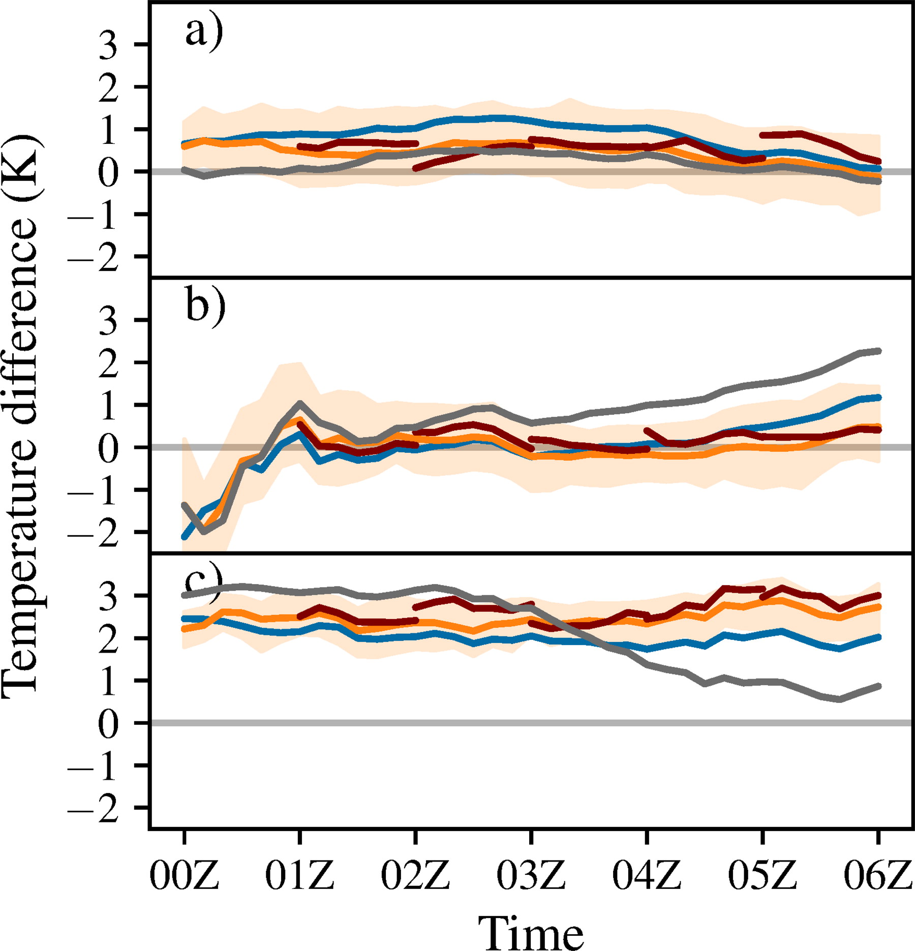
Fig. 8.
Time series of temperature differences between interpolated model output and observations in 50 meter height for all three test cases (a for 07 June 2016, b for 25 October 2016 and c for 12 November 2016). Four different colours show four different types of forecast (Blue: CONTROL experiment without assimilation; Orange: six-hour forecast started with analysis of WIND experiment at 0000 UTC; Red: analysis cycle of WIND experiment; Grey: six-hour forecast started with analysis of ALL experiment at 00 UTC). Solid lines display the ensemble mean, while orange tubes are the ensemble spread based on 5% and 95% percentile of WIND experiment’s control forecast.

Fig. 9.
Modelled and observed wind speed (FF, a, b & c) and potential temperature (TP, d, e and f) at 0300 UTC for 07 June 2016 (a & d), for 25 October 2016 (b & e), and for 12 November 2016 (c & f). Transparent orange lines are 40 ensemble members from forecast of WIND experiment based on analysis at 0000 UTC, while the ensemble mean from this forecast is shown as bold orange lines with crosses as marker. The blue line is the ensemble mean CONTROL experiment, while the forecast of the ALL experiment is displayed in grey. The red line is the analysis of the WIND experiment at 0300 UTC, nudged towards the black observations.