
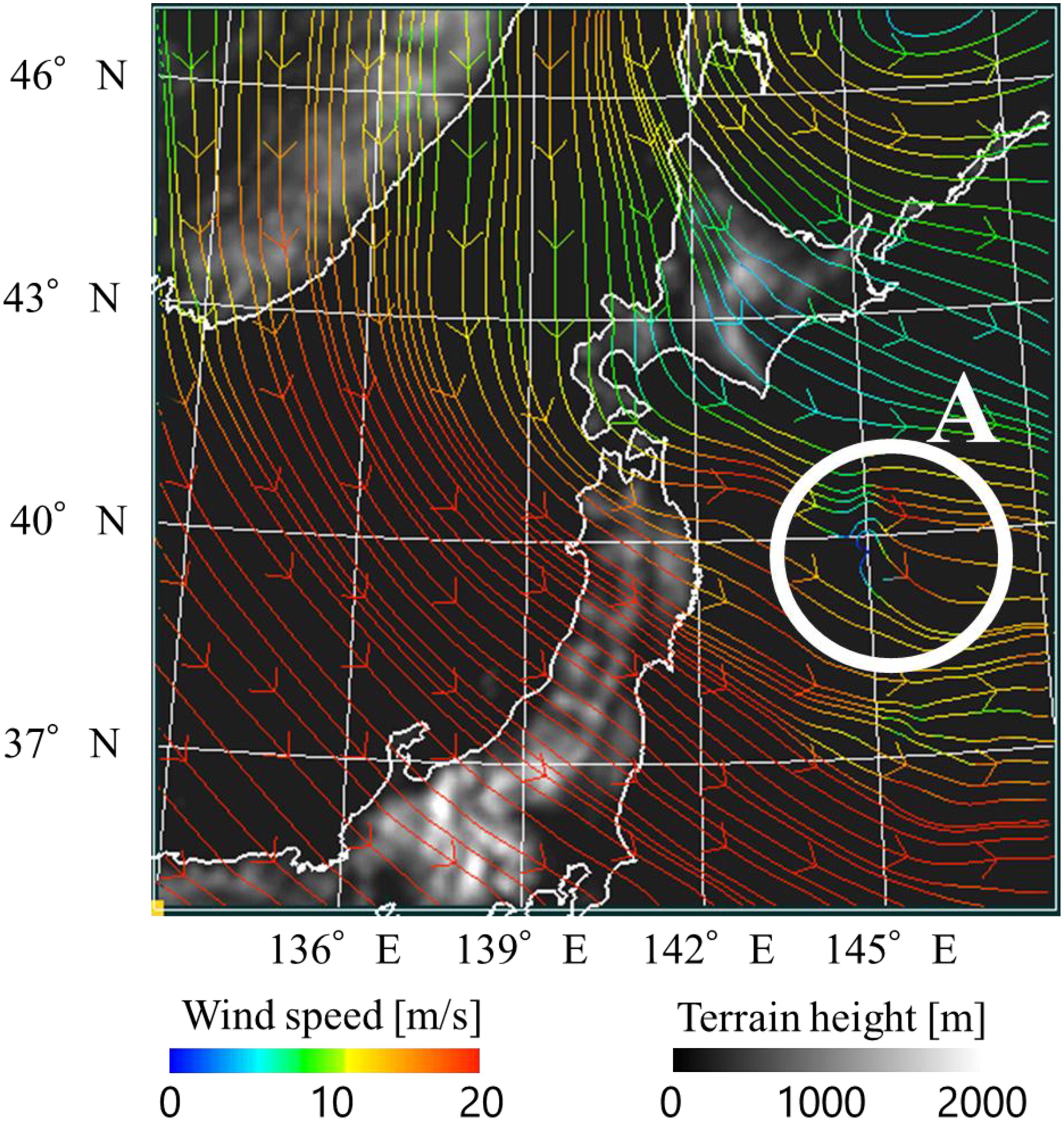
Fig. 1.
Computational domain, geographical height, and streamline at the assimilation time (2017/2/7 12:00 GMT) for level 12. The strong northwest wind observed in the figure is caused by a typical pressure pattern of winter in Japan. A small turbulence is found in circle A.
Table 1.
Conditions for the observability calculation.
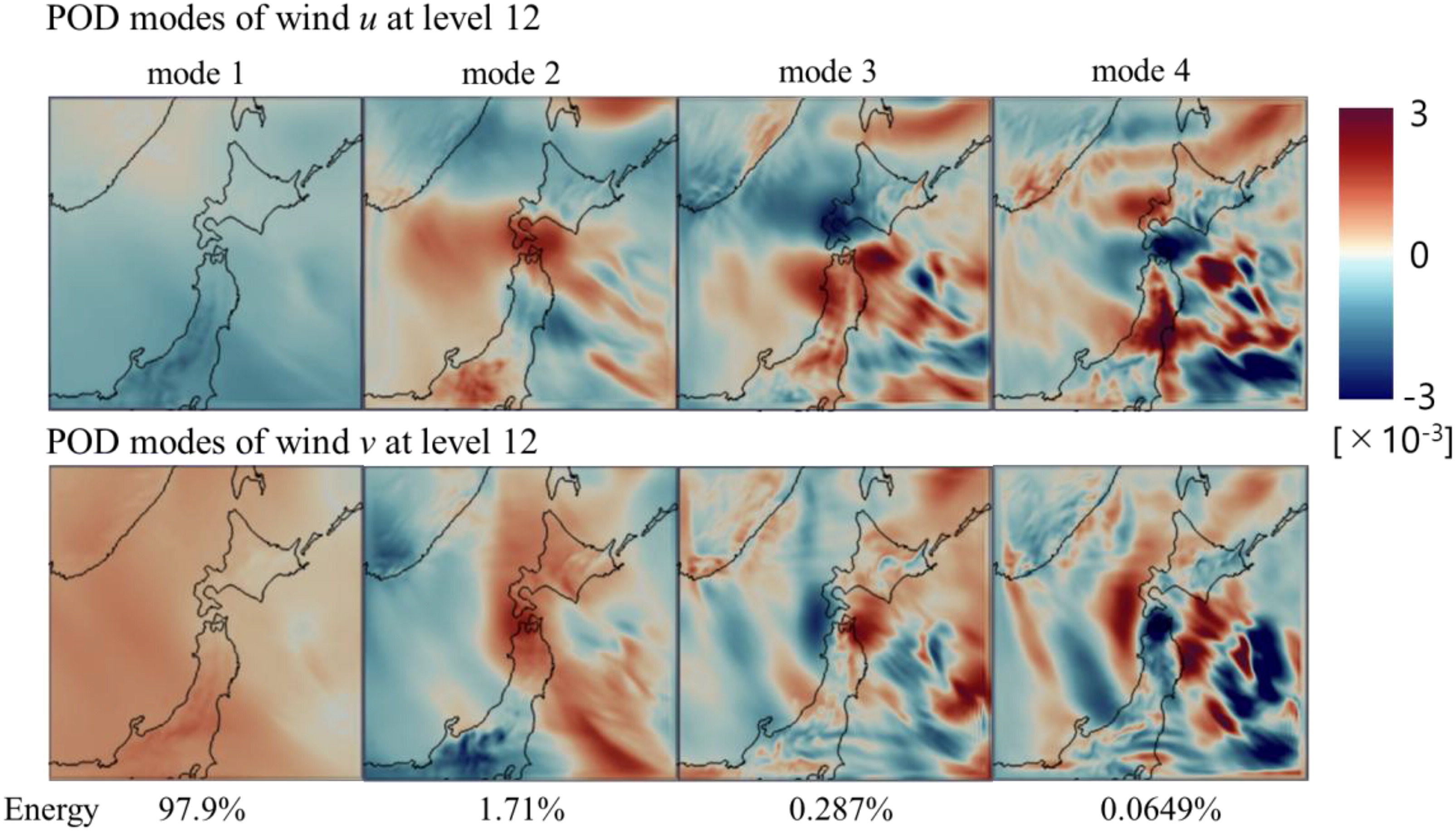
Fig. 2.
Proper orthogonal decomposition (POD) bases for wind components and at level 12. Each mode is normalised in whole domain.
Table 2.
Computational conditions for the identical-twin experiment.
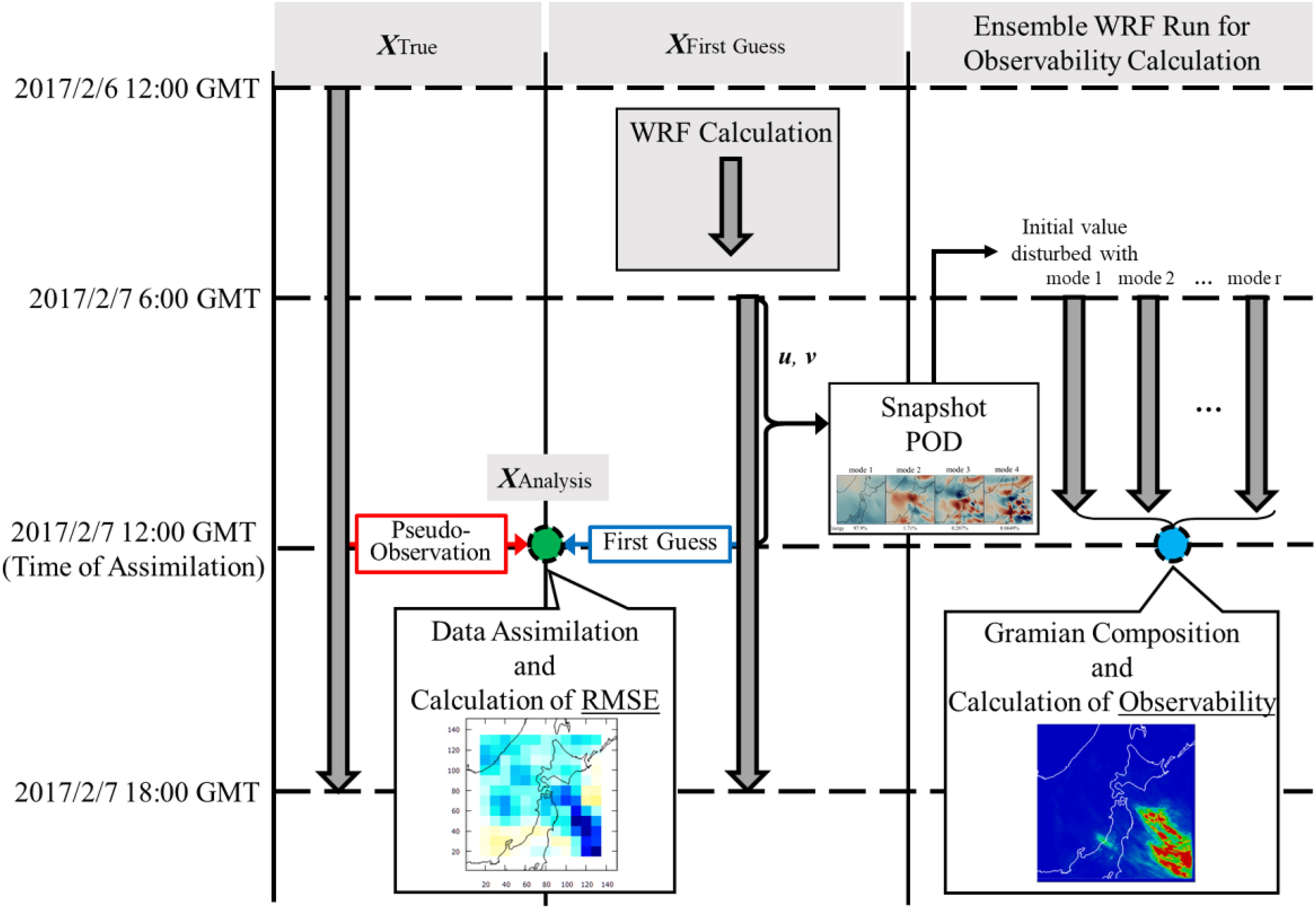
Fig. 3.
Schematic of identical-twin experiment and the calculation of observability.
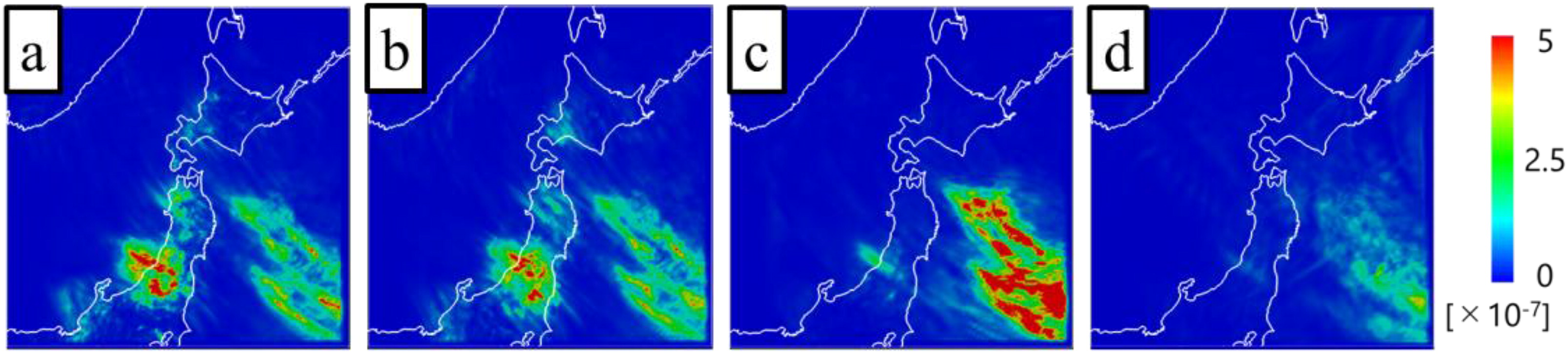
Fig. 4.
Spatial distribution of minimum eigenvalues at each level, where (a), (b), (c), and (d) correspond to the distribution at level 2 (150 m), 7 (850 m), 12 (3200 m) and 17 (8000 m), respectively.
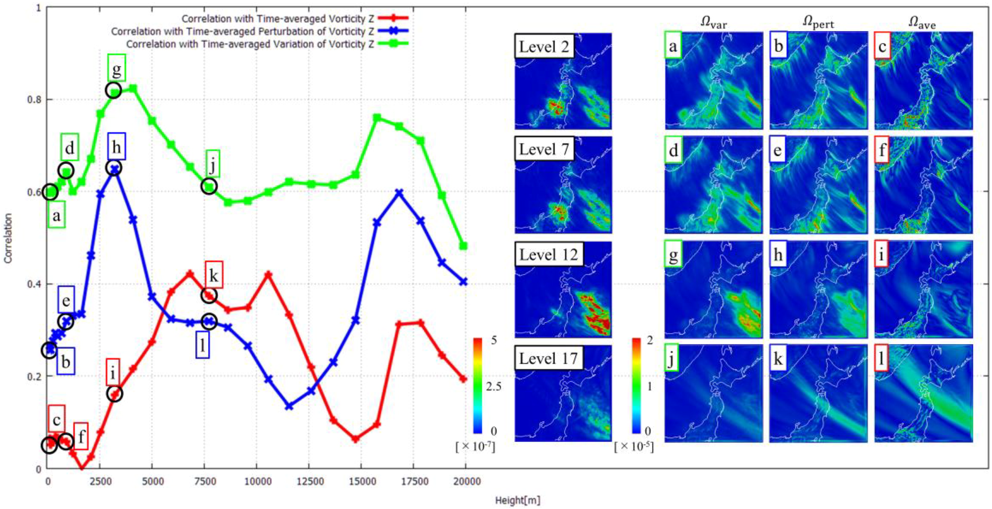
Fig. 5.
Correlations of the minimum eigenvalues and the actual distribution at levels 2, 7, 12, and 17. The vertical and horizontal axes correspond to the correlation coefficient and vertical height, respectively. The correlations with the time-averaged vorticity (red line), time-averaged perturbation of vorticity (blue line), and time-averaged temporal variation of vorticity (green line) are plotted. Each label on the left plot corresponds to the vorticity distributions on the right.
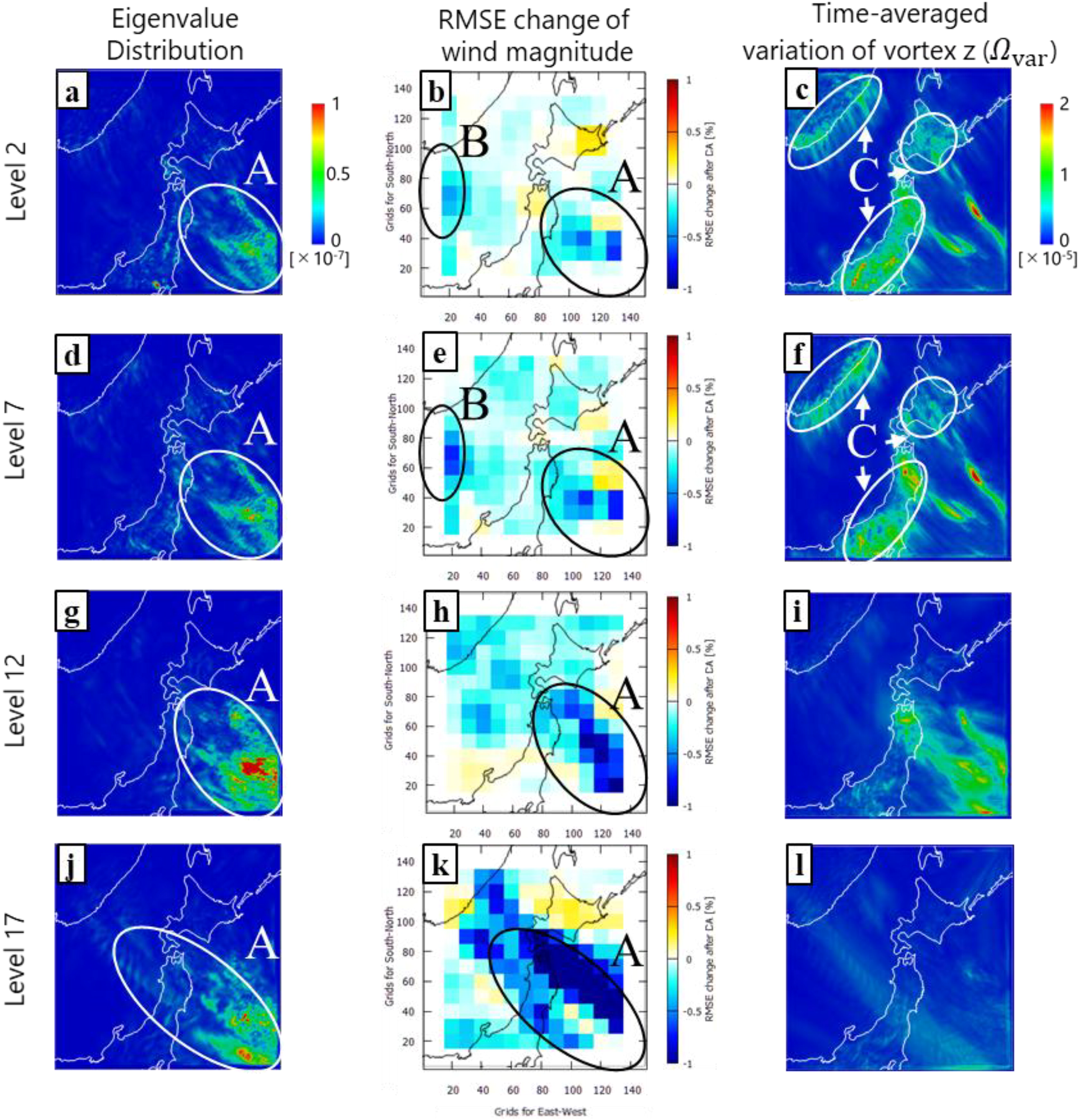
Fig. 6.
The distribution of eigenvalue, RMSE changes of wind magnitude, and time-averaged temporal variation of vorticity for levels 2, 7, 12, and 17, respectively. Area A shows the region where the correlation with the eigenvalue distribution is observed. Area B shows the region where RMSE reduction is observed regardless of almost zero eigenvalue. The first 6 h of the wind data (2017/2/7 6:00 GMT – 2017/2/7 12:00 GMT) are utilised to compose the Gramian.