
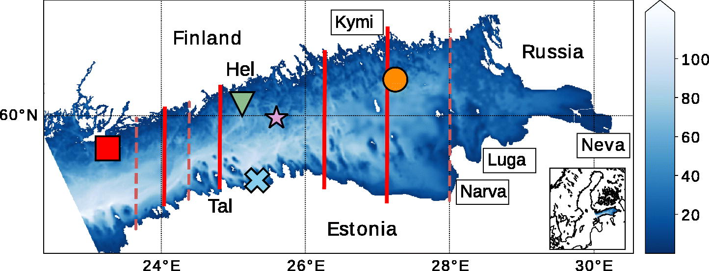
Fig. 1.
The model domain and bathymetry (in metres). CTD stations referenced in the article (from the east): Haapasaari (orange circle), Länsi-Tonttu (green triangle) and Längden (red square). Kalbådagrund weather station is marked with a magenta star. Station 18A used in analysis is marked with a blue X. Red lines show the location of the transects used in the analysis. Solid, darker lines indicate transects that were used for plots in this article. The map also indicates the approximate location of the Neva river mouth at the eastern end of the basin, along with Kymi, Luga and Narva rivers. Furthermore, approximate locations of the cities of Helsinki (Hel) and Tallinn (Tal) are shown. The inset is the location of the model domain on a map of the Baltic Sea.
Table 1.
Modelled daily average temperatures and salinities from the NEMO model compared against CTD observations, 2007–2013.
Table 2.
Wind forcing, RMS errors and biases (m/s).
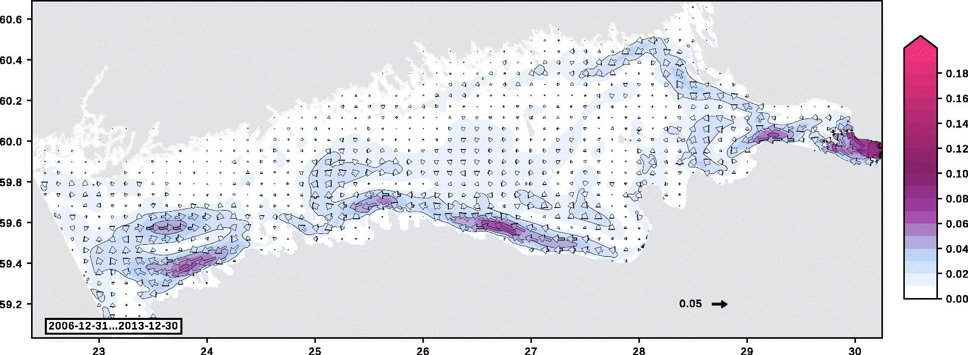
Fig. 2.
Annual mean circulation averaged from 0 to 7.5 m depth for the years 2007–2013. Velocities are in m/s. Vector arrows are drawn for every 15 grid points in the longitudinal direction and every 13 grid points in the latitudinal direction.
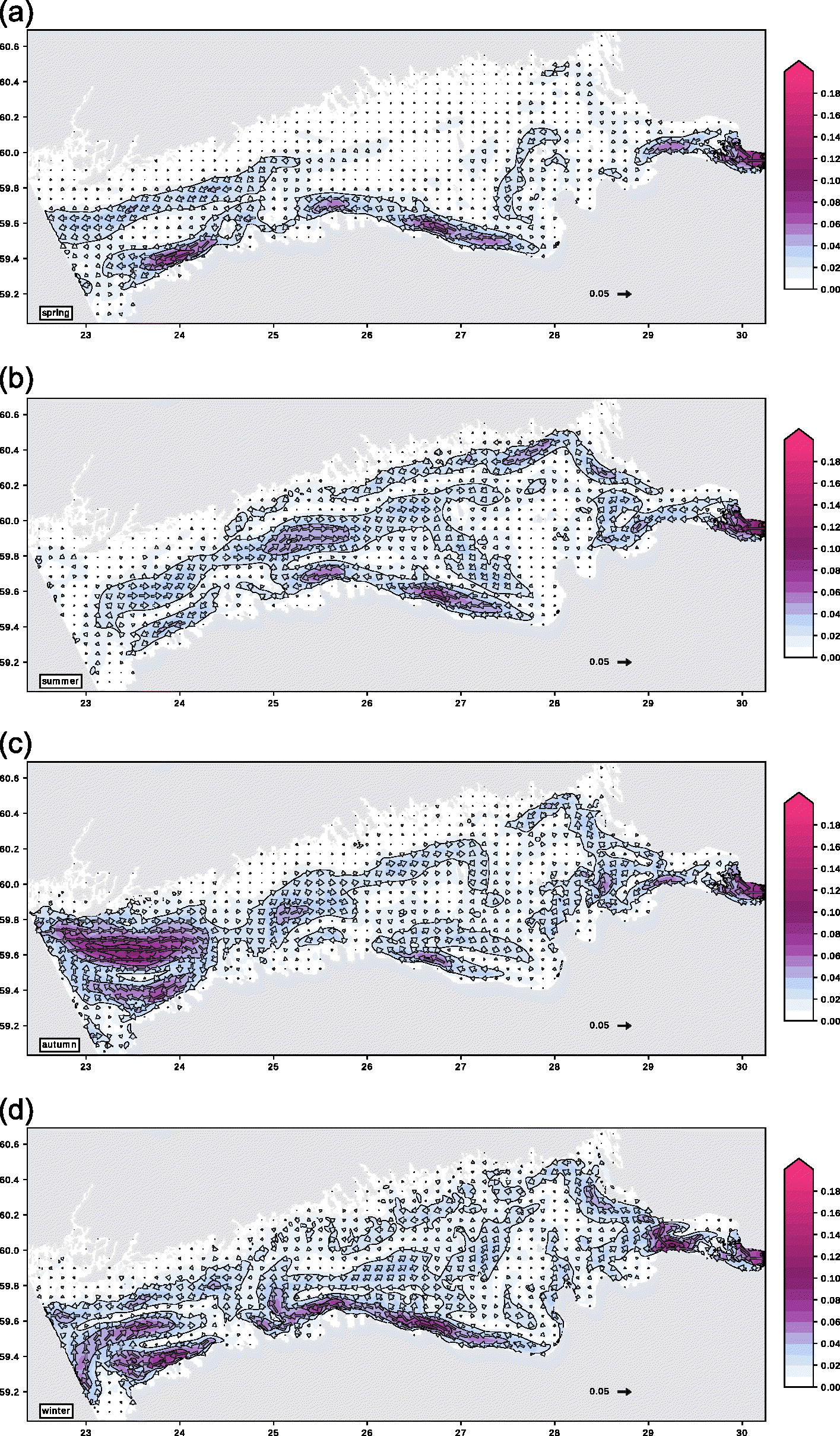
Fig. 3.
Mean circulation in 2007–2013 averaged from 0 to 7.5 m depth for spring (top), summer, autumn and winter (bottom). Velocities are in m/s. Vector arrows are drawn for every 15 grid points in the longitudinal direction and in every 13 grid points in the latitudinal direction.
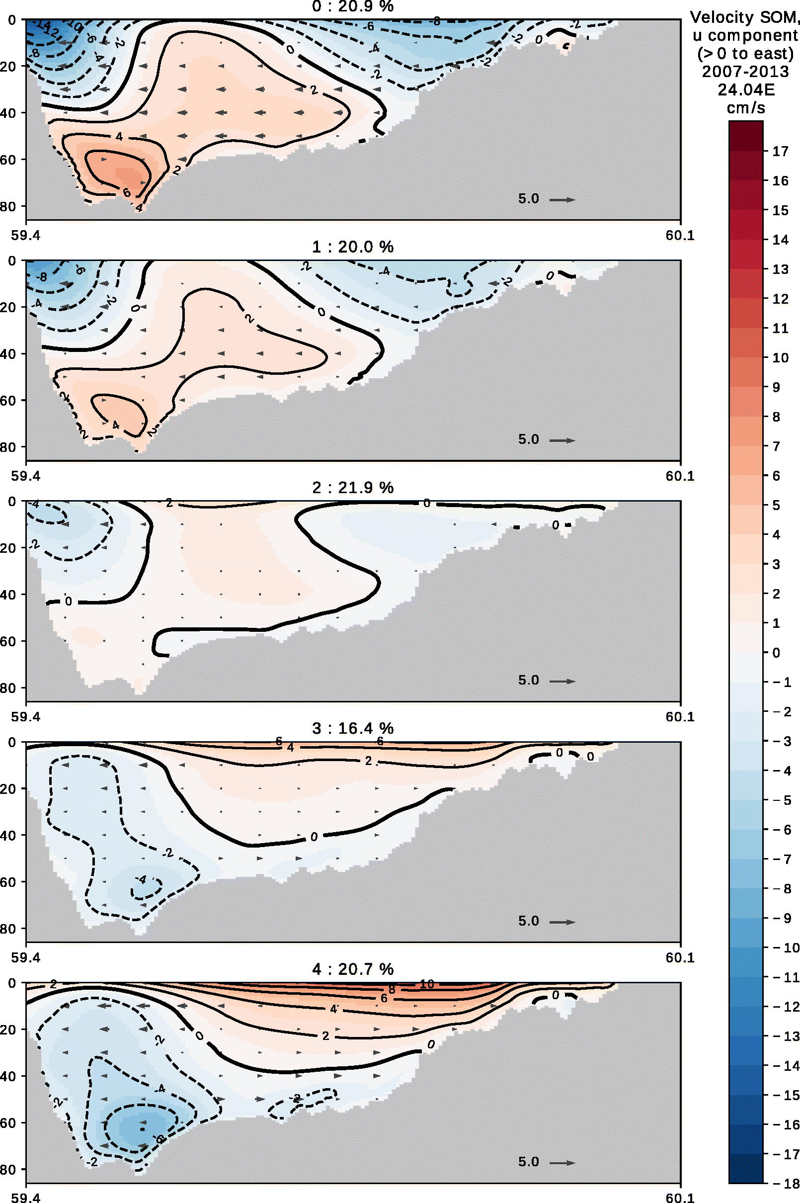
Fig. 4.
SOM patterns for modelled currents at a north-south section at 24.04°E. Data covers the years 2007–2013. Nodes are numbered from 0 to 4. Frequency of occurrence as percentages is indicated for each node. Colour contours indicate the u component of velocity, with positive values (red hues) for eastward velocities (into the page). Grey vector arrows show the v component of the velocity field, with every tenth vector displayed. Velocities are in cm/s.
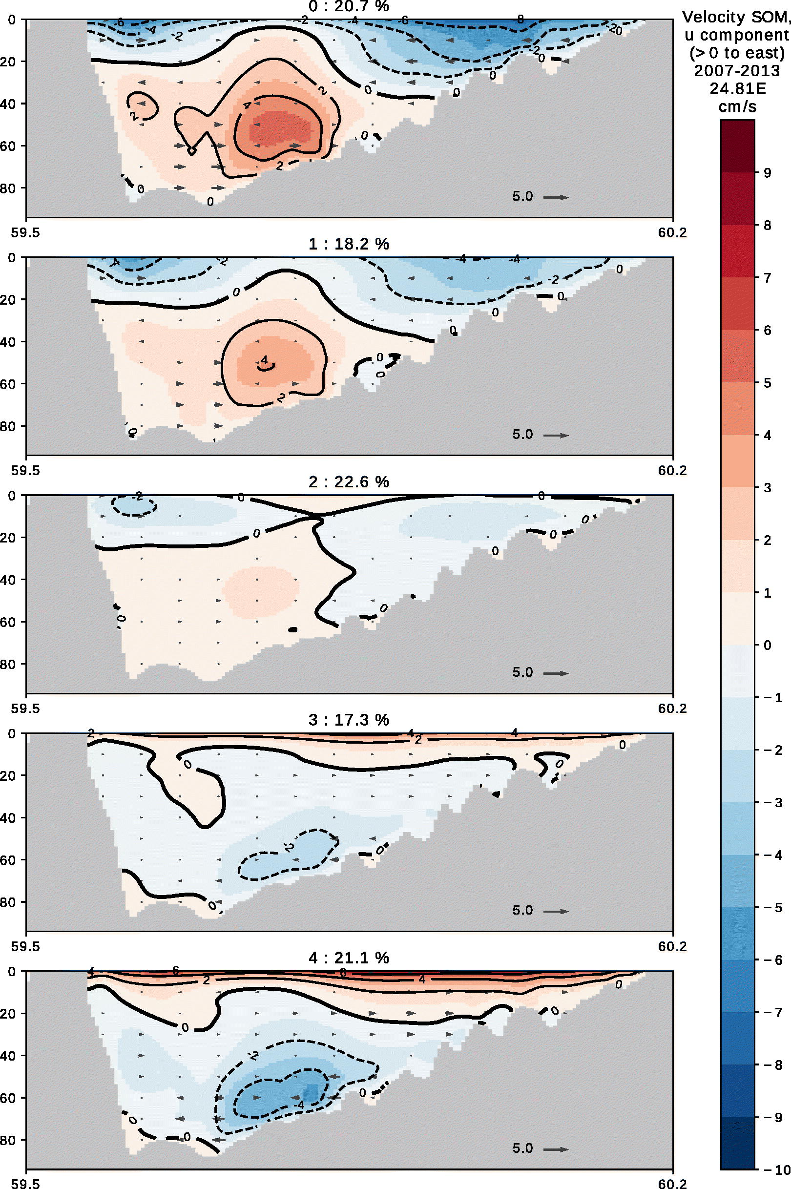
Fig. 5.
Like Fig. 4, but at 24.81°E.
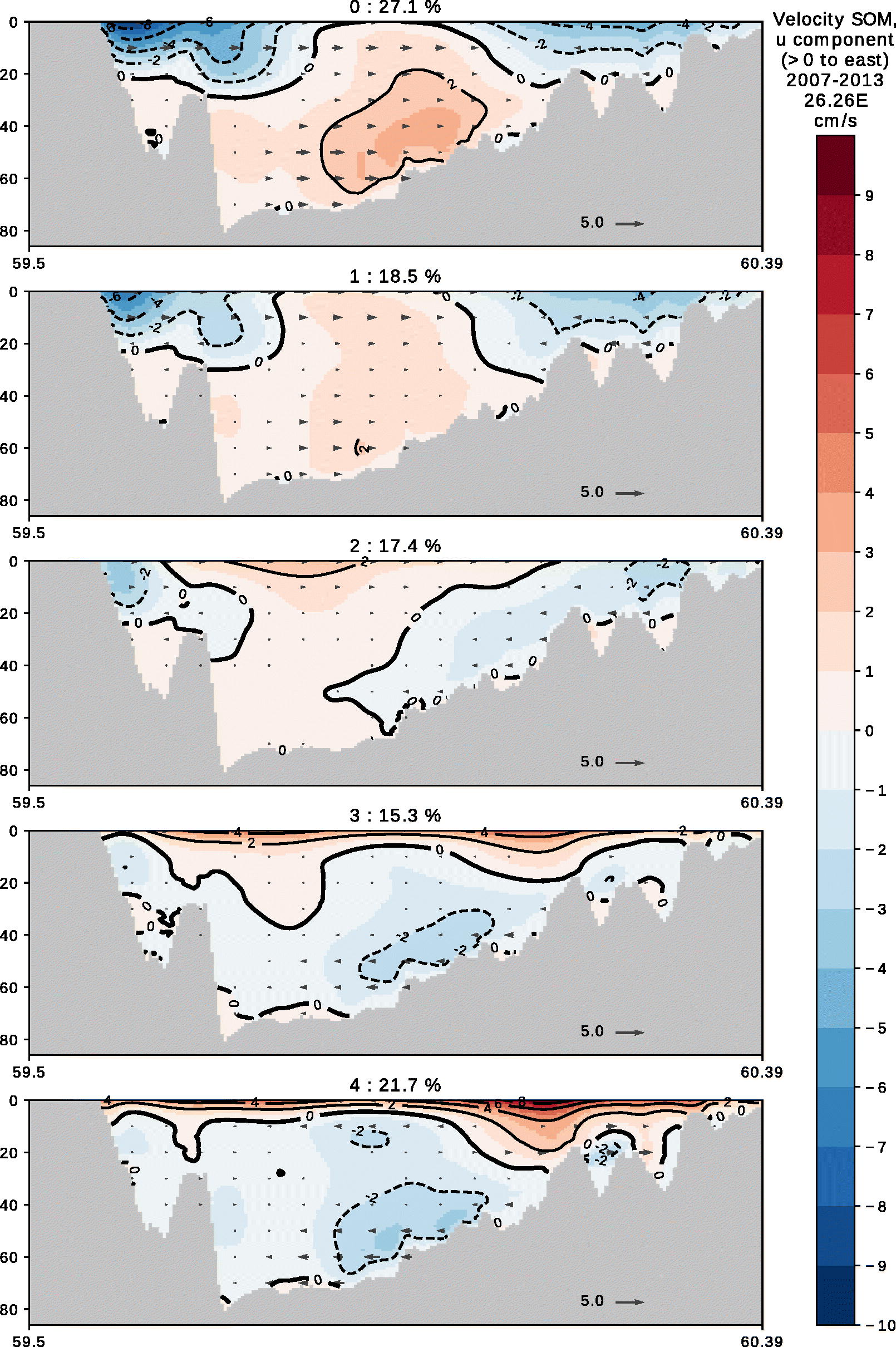
Fig. 6.
Like Fig. 4, but at 26.26°E.
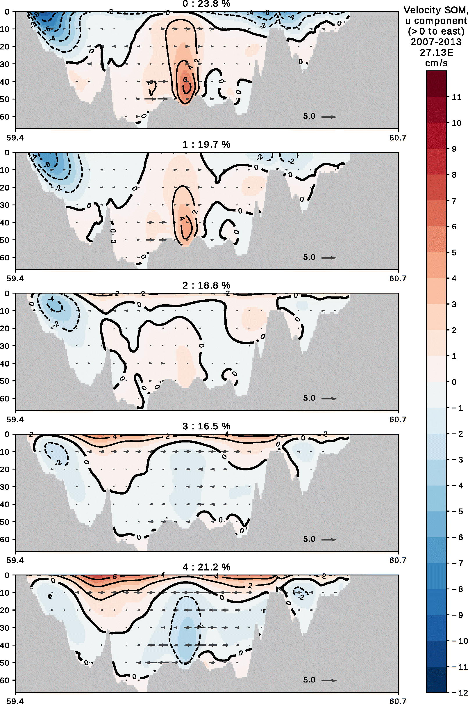
Fig. 7.
Like Fig. 4, but at 27.13°E.
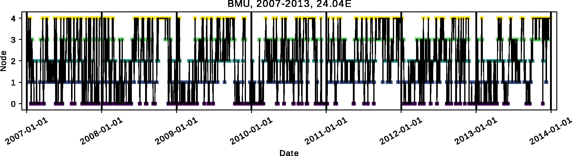
Fig. 8.
SOM BMU time series for the section in Fig. 4. Node numbers are the same as in Fig. 4.
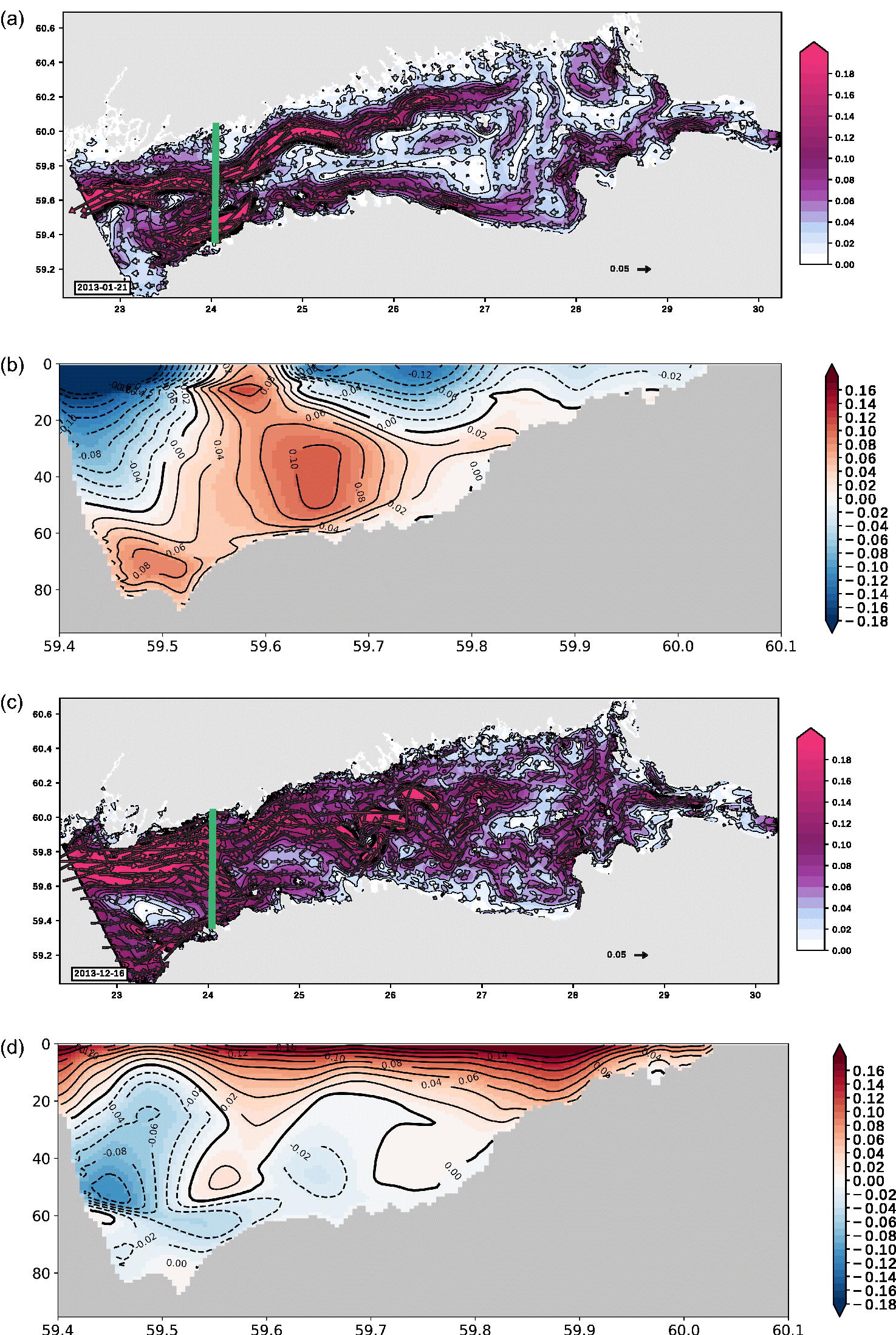
Fig. 9.
Daily mean velocity maps and zonal component of velocity at north-south section at 24.04°E for 21 January 2013 (normal estuarine circulation) and 16 December 2013 (reversed estuarine circulation). Vector arrows are drawn for every 19 grid points in the longitudinal direction and every 17 grid points in the latitudinal direction. Location of the north-south section is indicated by a green line on the velocity maps.
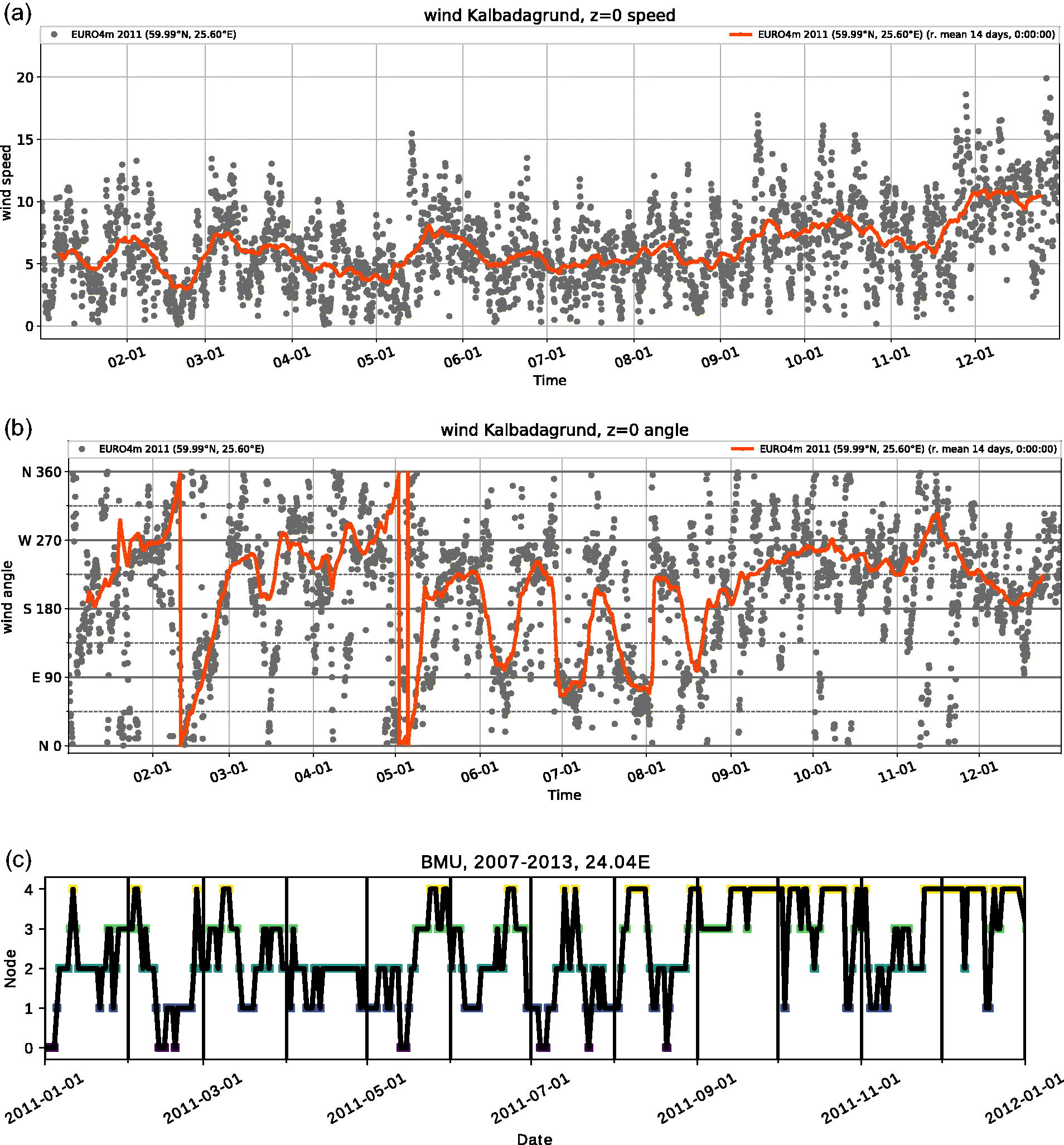
Fig. 10.
Top: wind speed and direction used as model forcing at Kalbådagrund, 2011 (black dots). 14-day running mean overlay (red line). Bottom: the BMU timeseries at 24.04°E for the same period. Wind vector averages were calculated component-wise.
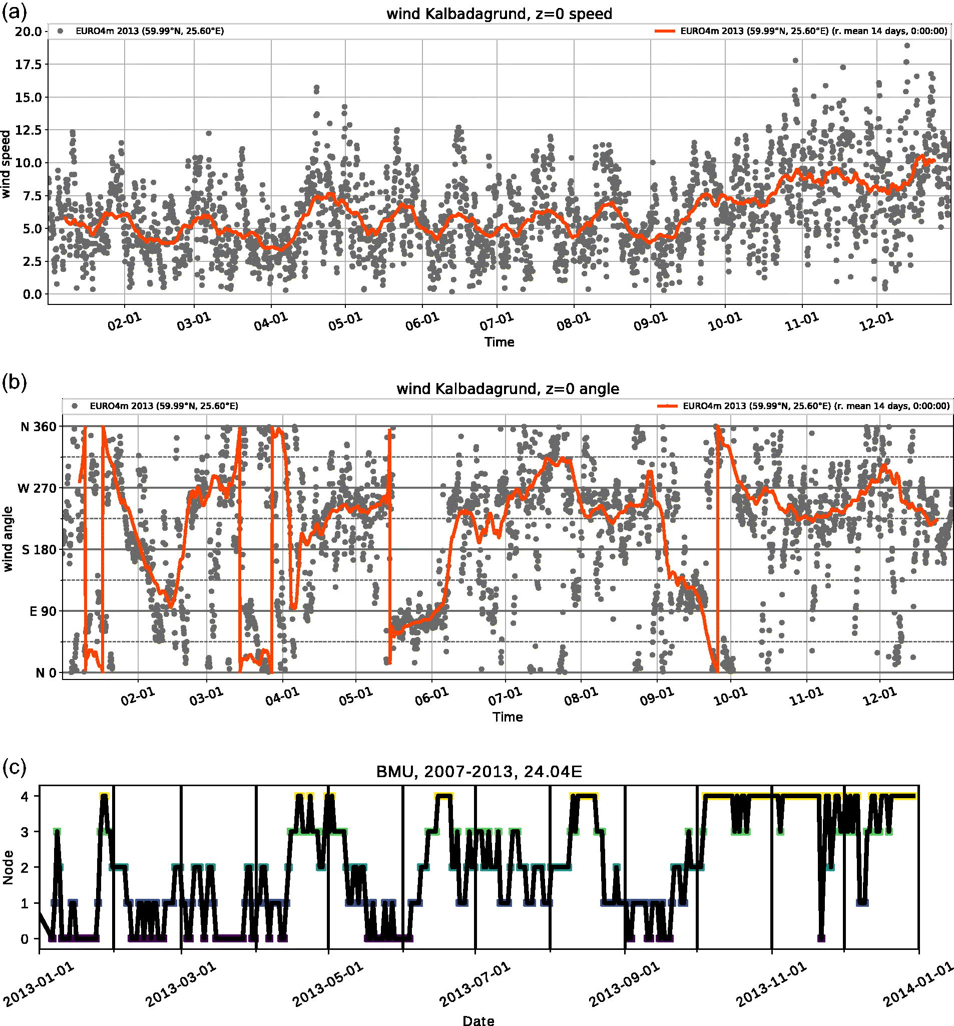
Fig. 11.
Like Fig. 10, but for 2013.
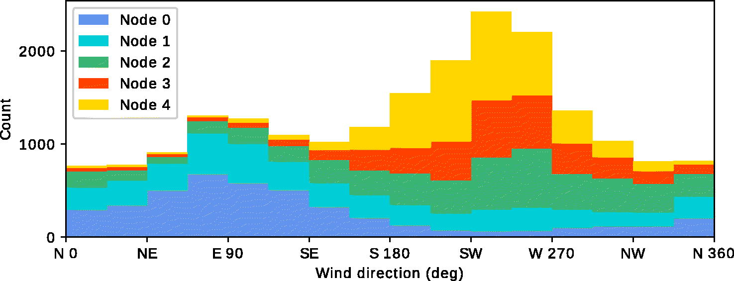
Fig. 12.
Wind direction distribution for BMU’s of SOM nodes as a stacked histogram, 2007–2013. Wind direction taken from the model forcing at the Kalbådagrund station. BMU from the section at 24.04°E.
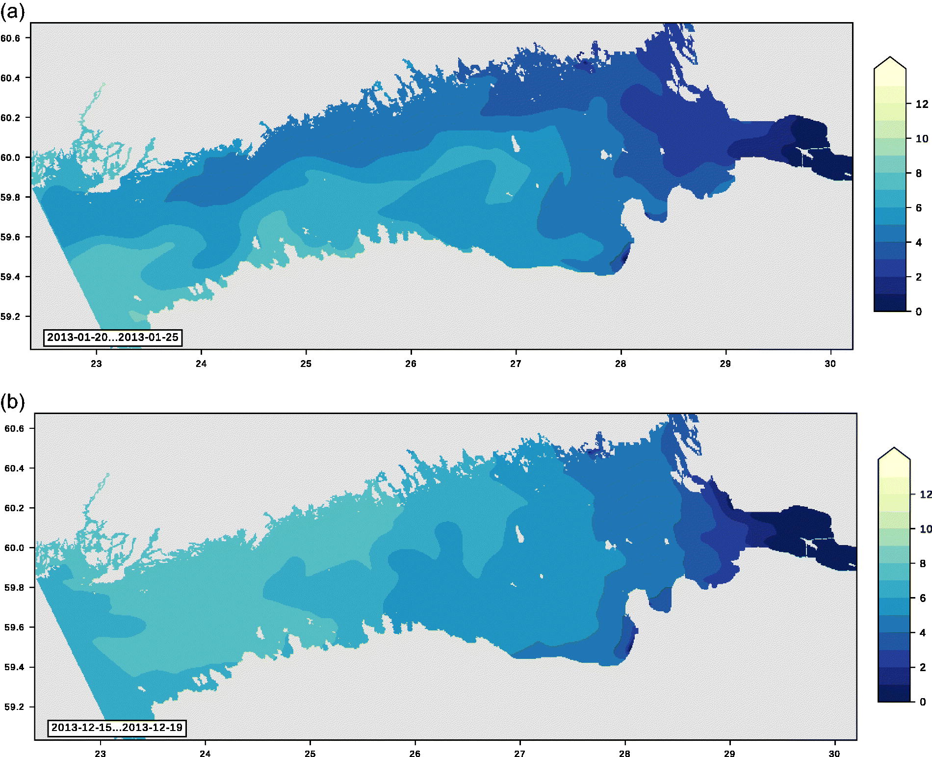
Fig. 13.
Mean surface salinity (PSU) in the model for late January 2013 and mid-December 2013 (cf. Fig. 9).
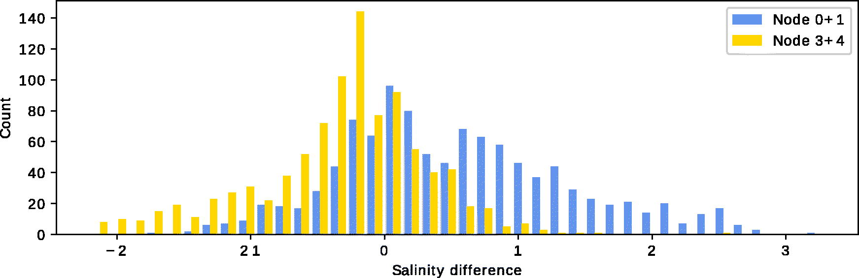
Fig. 14.
Histogram of modelled salinity (PSU) difference between northern and southern coast of GoF at 5 m depth, 2007–2013. Nodes 0 and 1 (normal estuarine circulation) and 3 and 4 (reverse estuarine circulation) are combined in this Figure. where is salinity at station 18 A near the southern coast and SLT at station Länsi-Tonttu near the northern coast (locations in Fig. 1).