
Table 1.
A short description of the datasets used in this study. The dataset and institution are given, as well as the time period and number of members (#) available. The underlying sea surface dataset is given in the penultimate column. A reference for each dataset is given in the last column.
Table 2.
Synoptic descriptions and abbreviations of the CAP9 (Cluster Analysis of Principal components with 9 types) and GWT10 (GrossWetterTypes with 10 types) circulation types.
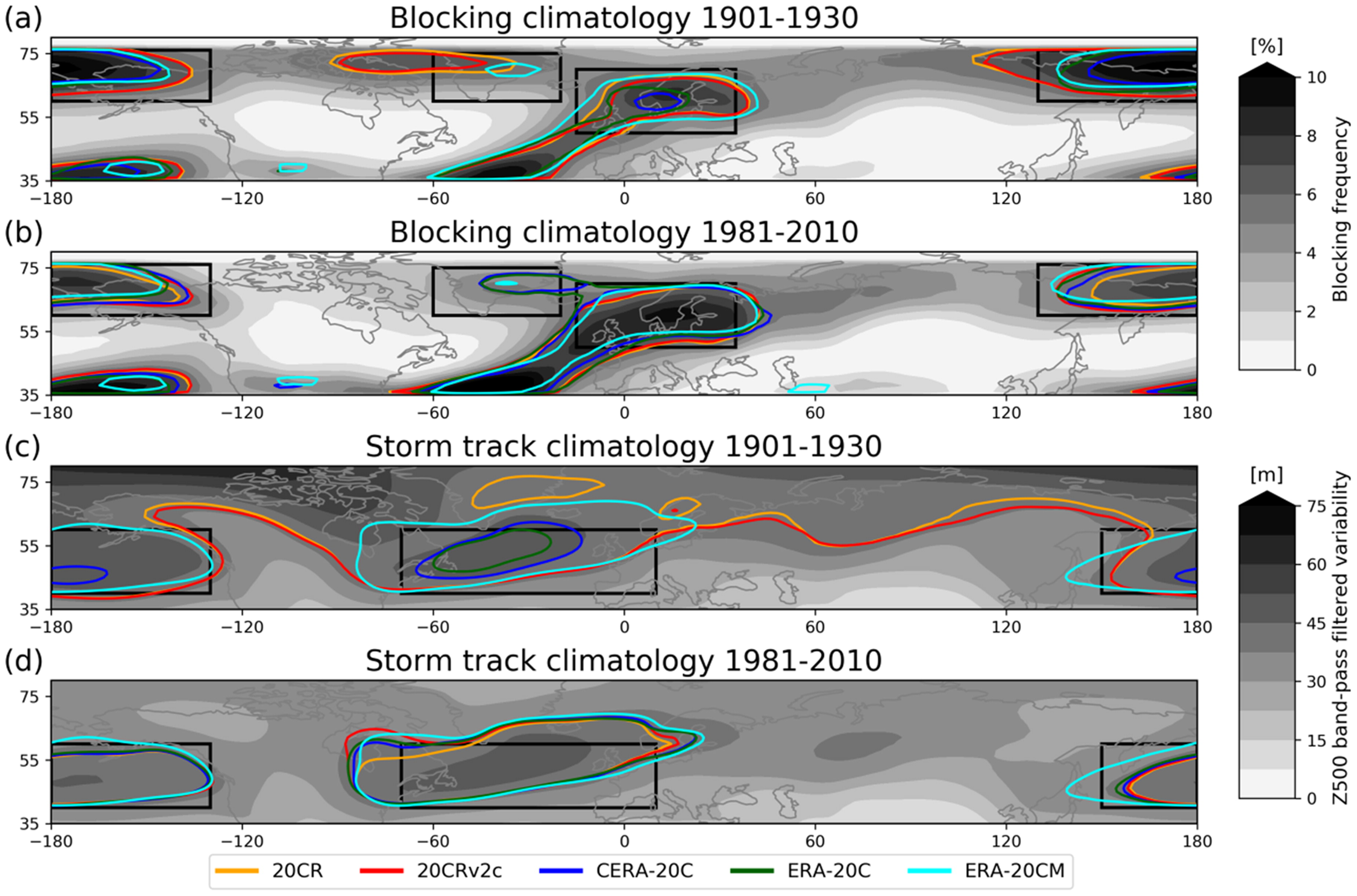
Fig. 1.
Annual mean distribution of the storm track (given by the mean storm track activity [m] in the early 20th century (1901–1930,a) and present (1981–2010,b). Panel c and d show the annual mean distribution of blocks (given by the blocking frequency [%/year]) in the early 20th century and present, respectively. The filled grey-scale contour denotes the climatological fields in 20CR. The coloured contours denote the 6% blocking frequency contour and the 50 m band-pass filtered 500 hPa geopotential height variability contour. The rectangles depict the subdomains used in this study. For blocks: Greenland (20°–60°W, 60°–75°N), Scandinavia (15°W–40°E, 50°–70°N), NPA (130°–230° E, 60°–75°N). For storm tracks: NAE (70°W–10°E, 40° –60°N), NPA (150°–230°E, 40°–60°N).
Table 3.
Definition of regions used in this study and the metric for which they are used. The last two columns provide the linear trend between 1950 and 2010 [%/100 years for blocks, m/100 years for STA] for the specific region and metric in winter (DJF) and summer (JJA). The five numbers are ordered as follows: 20CR, 20CRv2c, ERA-20C, CERA-20C, ERA-20CM.
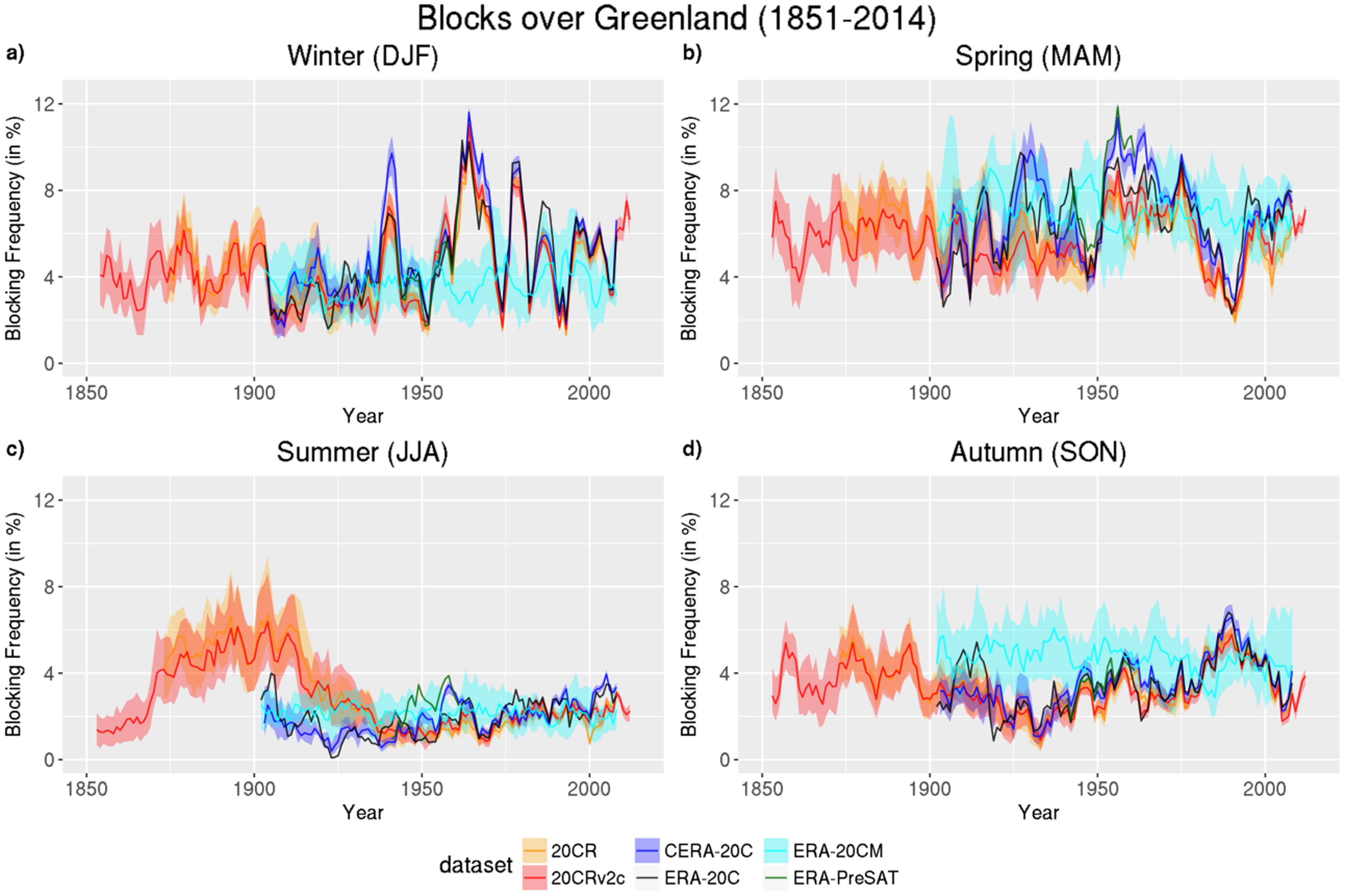
Fig. 2.
Seasonal blocking frequencies [fraction of blocked time steps in %] over the Greenland domain (60°–75°N, 20°–60°W) between 1851 and 2014. A 5-year running mean is applied for better readability. For multi-member datasets, the mean and the 10th and 90th percentiles are shown.

Fig. 3.
Correlation coefficients of the seasonal blocking frequency between two datasets over the Greenland domain (a) and the seasonal storm track activity over the NAE domain (b) between 1901 and 2010. The four numbers denote the correlation coefficient in winter (DJF, upper left), spring (MAM, upper right), summer (JJA, lower left) and autumn (SON, lower right).
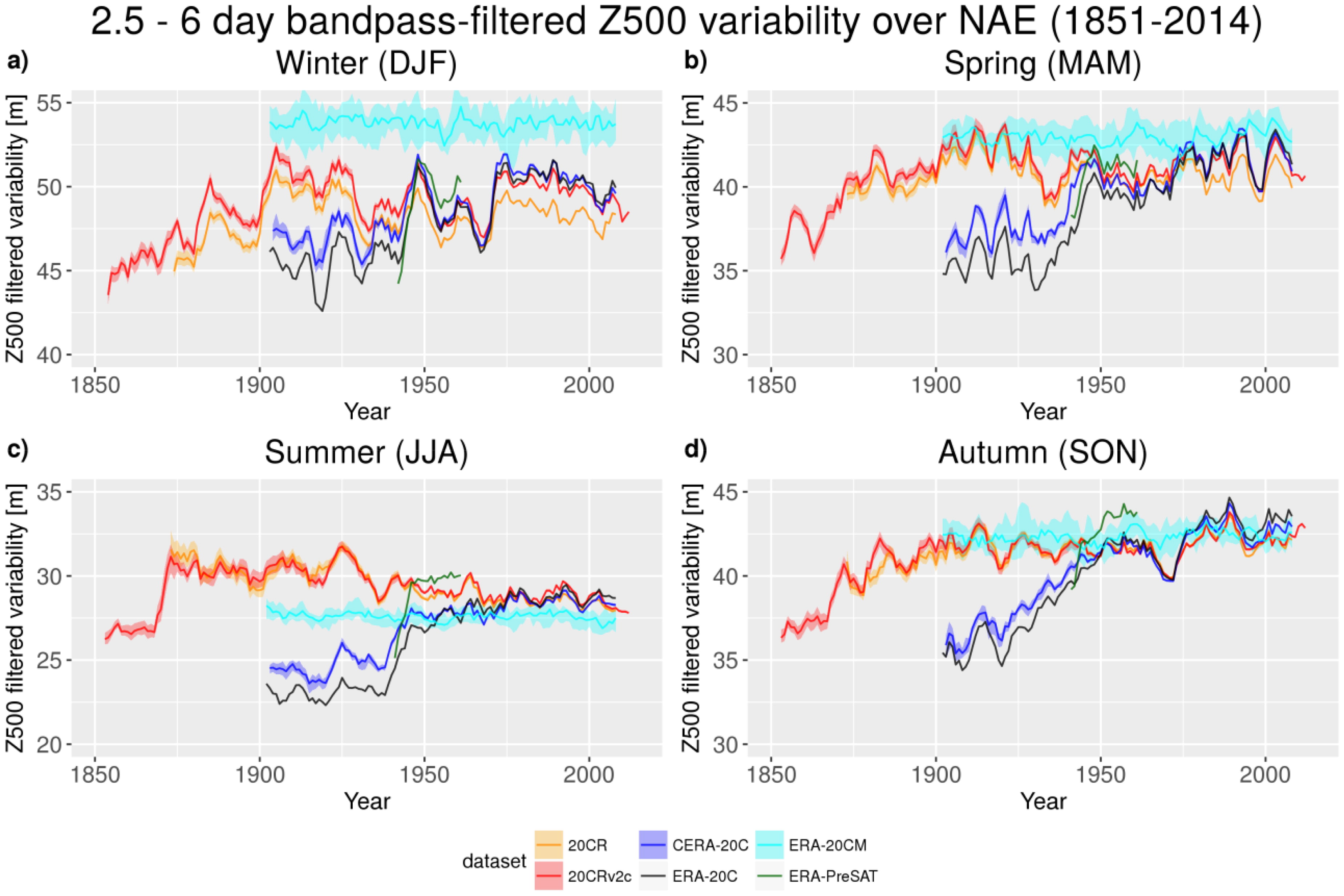
Fig. 4.
Storm track activity (500 hPa geopotential height band-pass filtered variability [m]) over the North Atlantic/European domain (40°–60°N, 70°W–10°E) between 1851 and 2014. For multi-member datasets, the multi-member mean and the 10th and 90th percentiles are shown. Note that the y-axis is different for each panel in order to present results in greater detail.
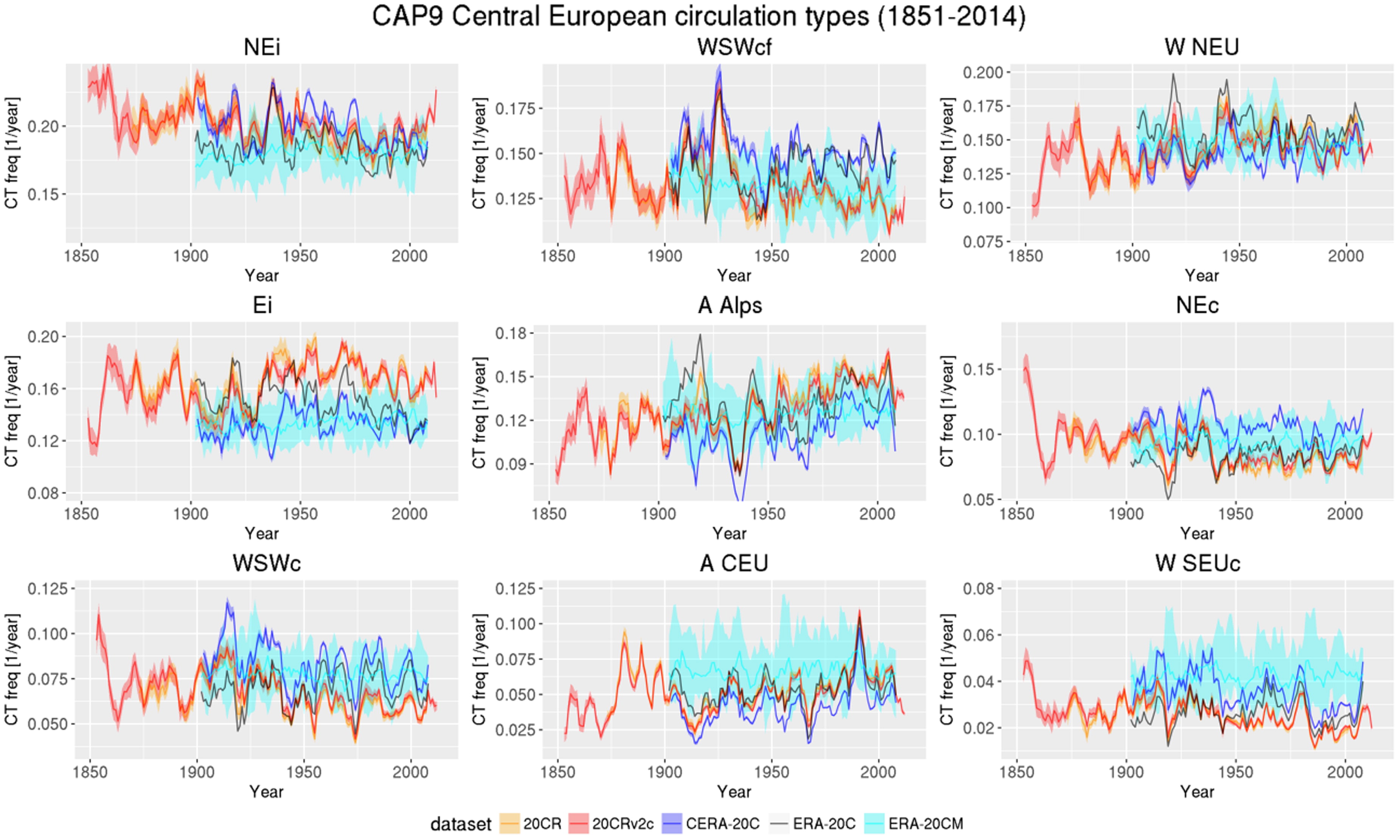
Fig. 5.
Annual circulation type frequency over the Alpine domain (41°–52°N, 3–20°E) between 1851 and 2014 for CAP9 (Cluster Analysis of Principal components with 9 types). A 5-year running mean is applied for better readability. For multi-member datasets, the mean and the 10th and 90th percentiles are shown.
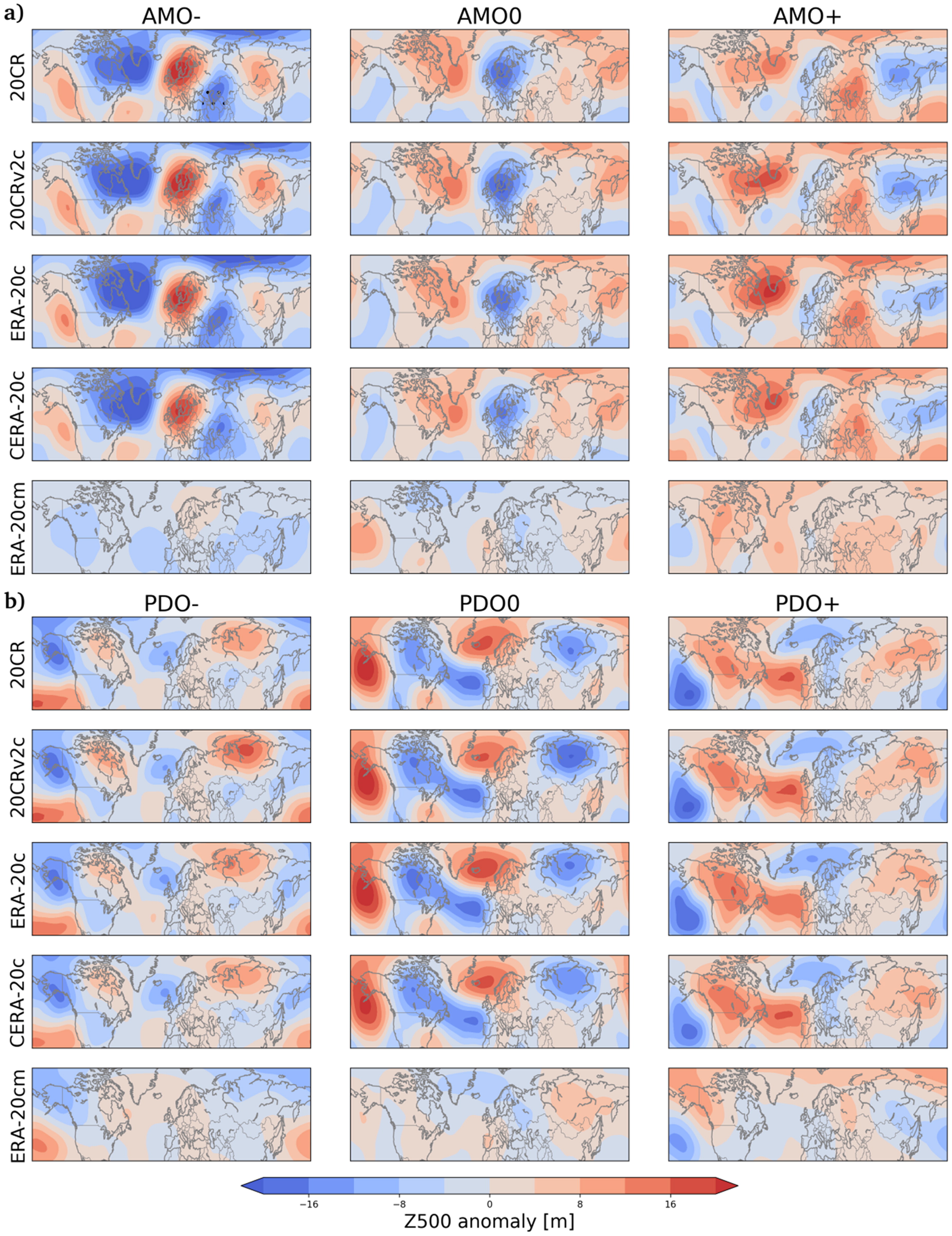
Fig. 6.
The winter (DJF) 500 hPa geopotential height anomalies during the negative (left), neutral (middle), and positive (right) terciles of the AMO (upper half) and PDO (lower half) between 1950 and 2010. Four surface-input reanalyses (20CR, 20CRv2c, ERA-20C and CERA-20C) and the ERA-20CM model simulation are shown. In case of multi-member datasets, the multi-member mean is shown. No significant anomalies (determined by the 95% CI) were found in any of the panels using the FDB (Wilks, 2016) and 20 000 bootstrap iterations.
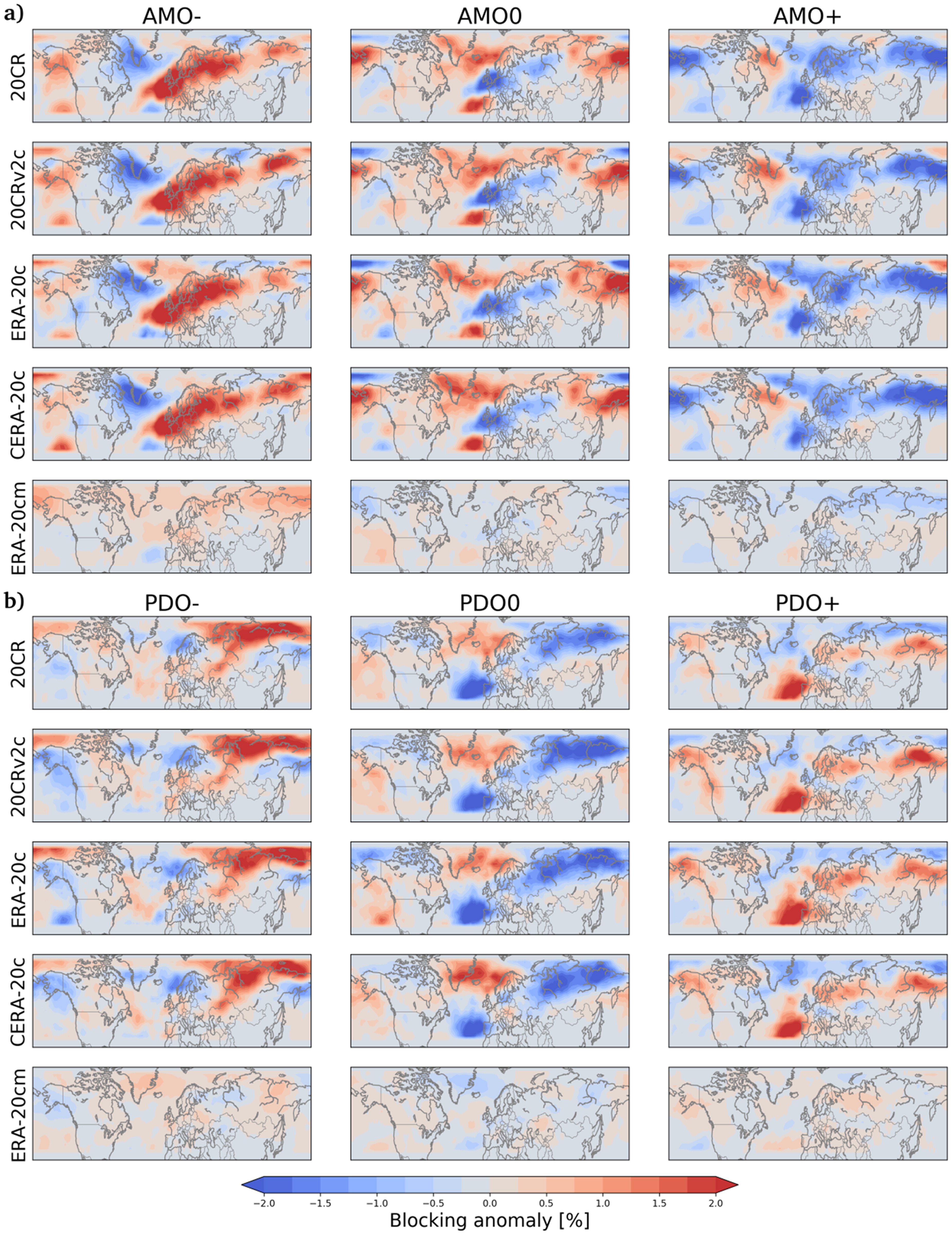
Fig. 7.
The winter (DJF) blocking anomalies during the negative (left), neutral (middle), and positive (right) terciles of the AMO (upper half) and PDO (lower half) between 1950 and 2010. In case of multi-member datasets, the multi-member mean is shown. No significant anomalies(determined by the 95% CI) were found in any of the panels using the FDB (Wilks, 2016) and 20 000 bootstrap iterations.

Fig. 8.
The winter (DJF) storm track anomalies during the negative (left), neutral (middle), and positive (right) terciles of the AMO (upper half) and PDO (lower half) between 1945 and 2010. In case of multi-member datasets, the multi-member mean is shown. The stippling denotes areas with significant anomalies(determined by the 95% CI) after applying the FDR (Wilks, 2016) and 20 000 bootstrap iterations.
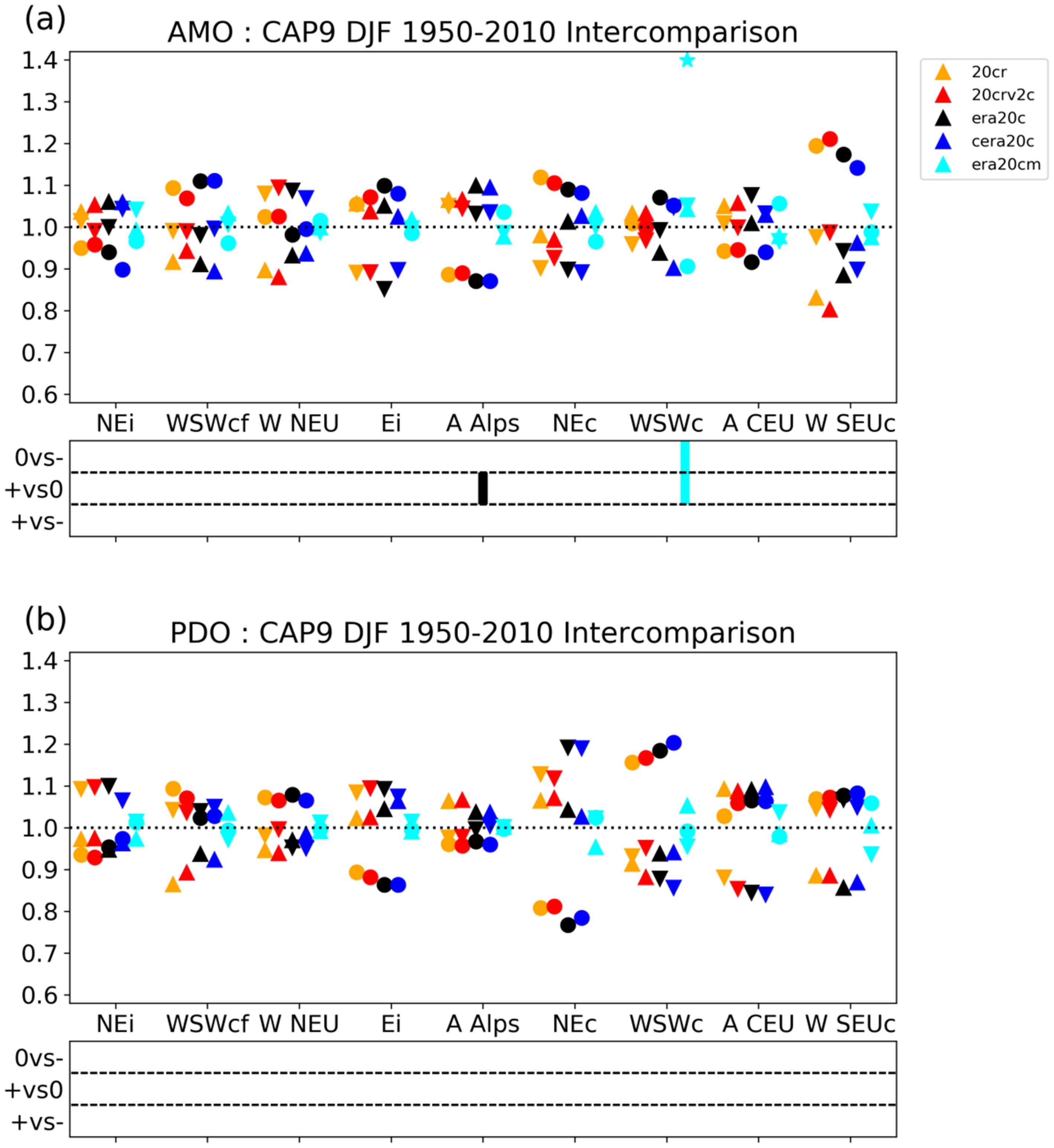
Fig. 9.
Normalized circulation type frequencies for CAP9 (Cluster Analysis of Principal components with 9 types) during high (triangle facing up), neutral (circle), or low (triangle facing down) AMO (upper half) and PDO (lower half) indices between 1950 and 2010 in winter (DJF). Different reanalyses (20CR orange, 20CRv2c red, CERA-20c blue, and ERA-20c black) and the ERA-20CM model simulation (cyan) are depicted. For multi-member datasets, the multi-member mean is shown. The lower panel shows significant differences between the neutral and negative terciles (upper row), the positive and neutral terciles (middle row), and the positive and negative terciles (lower row). Significance is tested with a Welch’s t-test augmented to account for autocorrelation (e.g. Wilks, 2006). See Table 1 for a short description of the circulation types.