
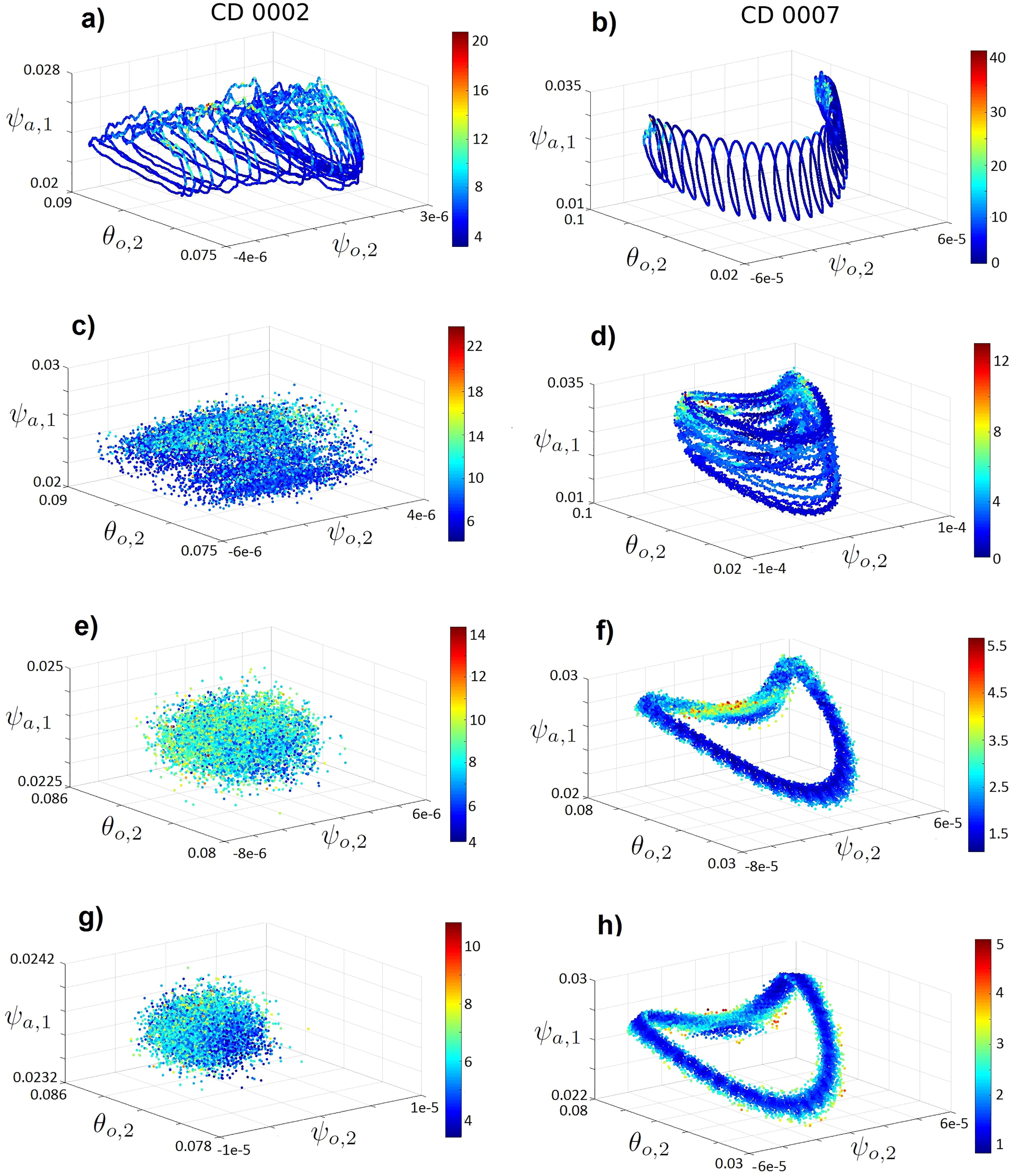
Fig. 1.
Poincaré sections for the modes and . Different couplings (a,c,e,g): C = 0.002. (b,d,f,h) C = 0.007. Different averaging windows: (a,b) daily; (c,d) monthly; (e,f) yearly and (g,h) 8-year averages.
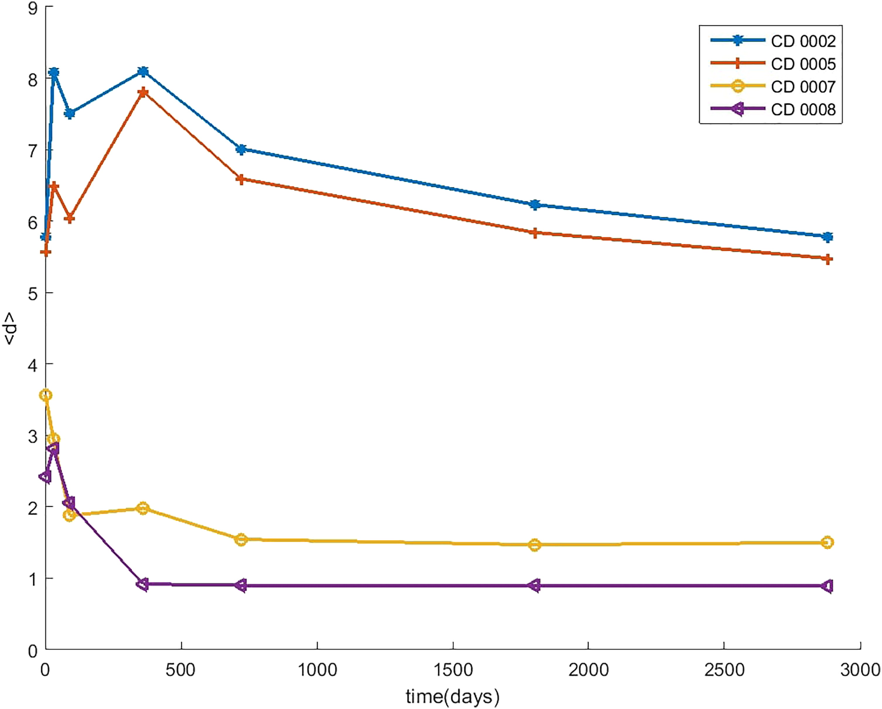
Fig. 2.
Attractor dimensions as a function of the coupling and the averaging window.
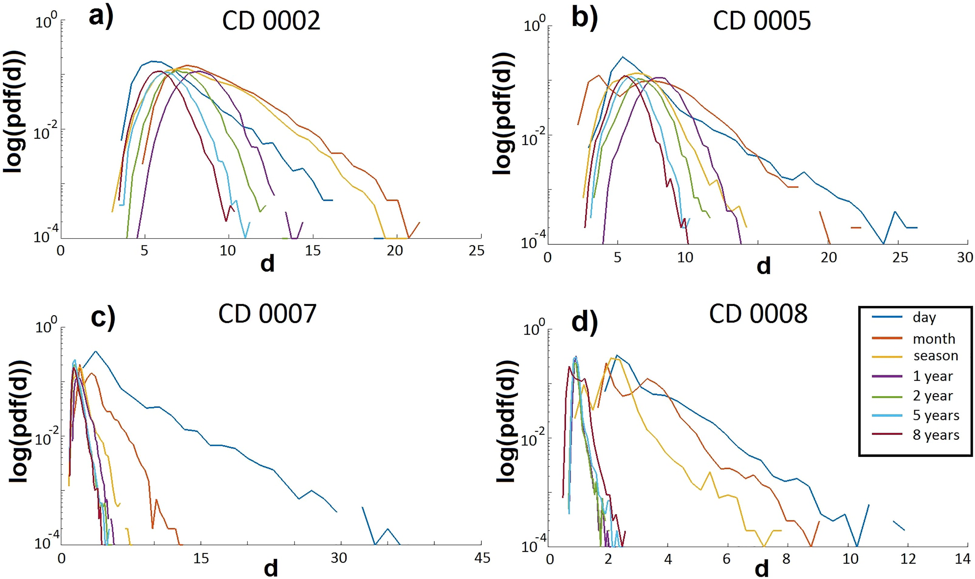
Fig. 3.
Attractor dimensions’ probability density functions (pdfs) vs coupling coefficient C and averaging window. (a) C = 0.002, (b) C = 0.005, (c) C = 0.007 and (d) C = 0.008.
Table 1.
Moments of the probability density functions (pdf) of d for different C and averaging windows.
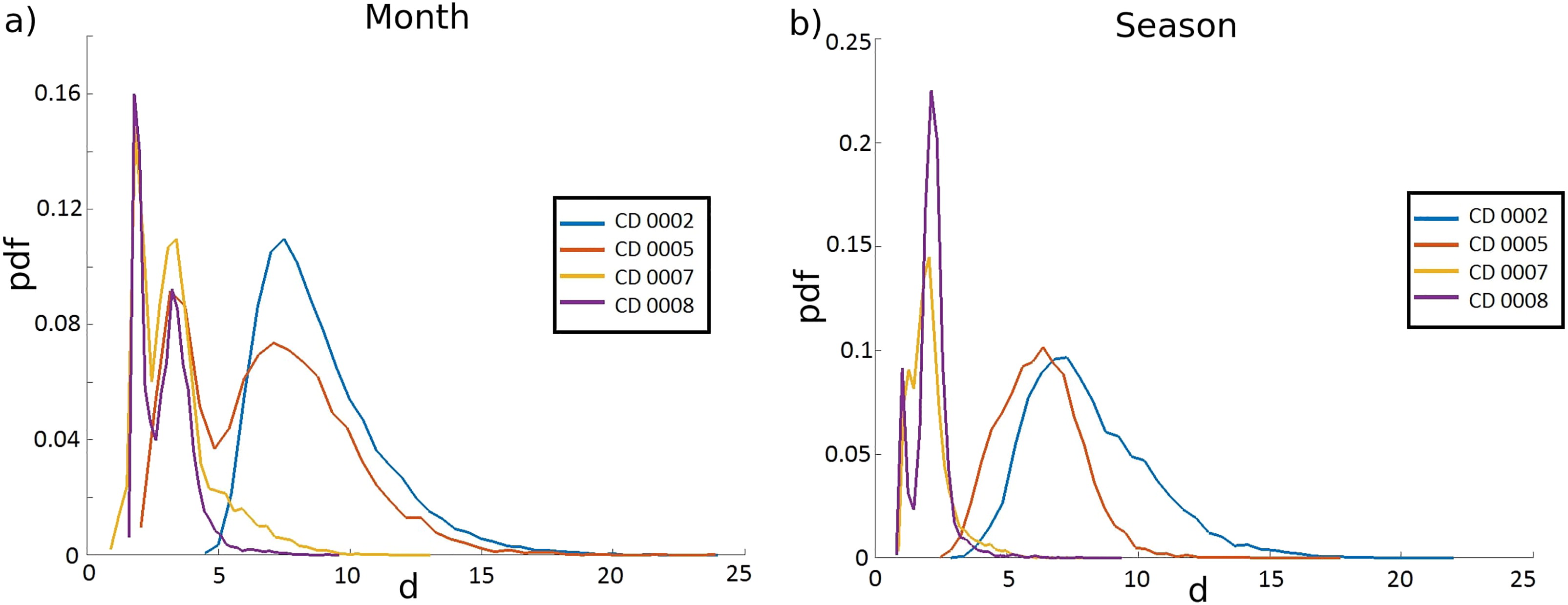
Fig. 4.
Attractor dimensions’ probability density functions (pdfs) vs coupling coefficient C for monthly (a) and seasonal (b) averaging windows.
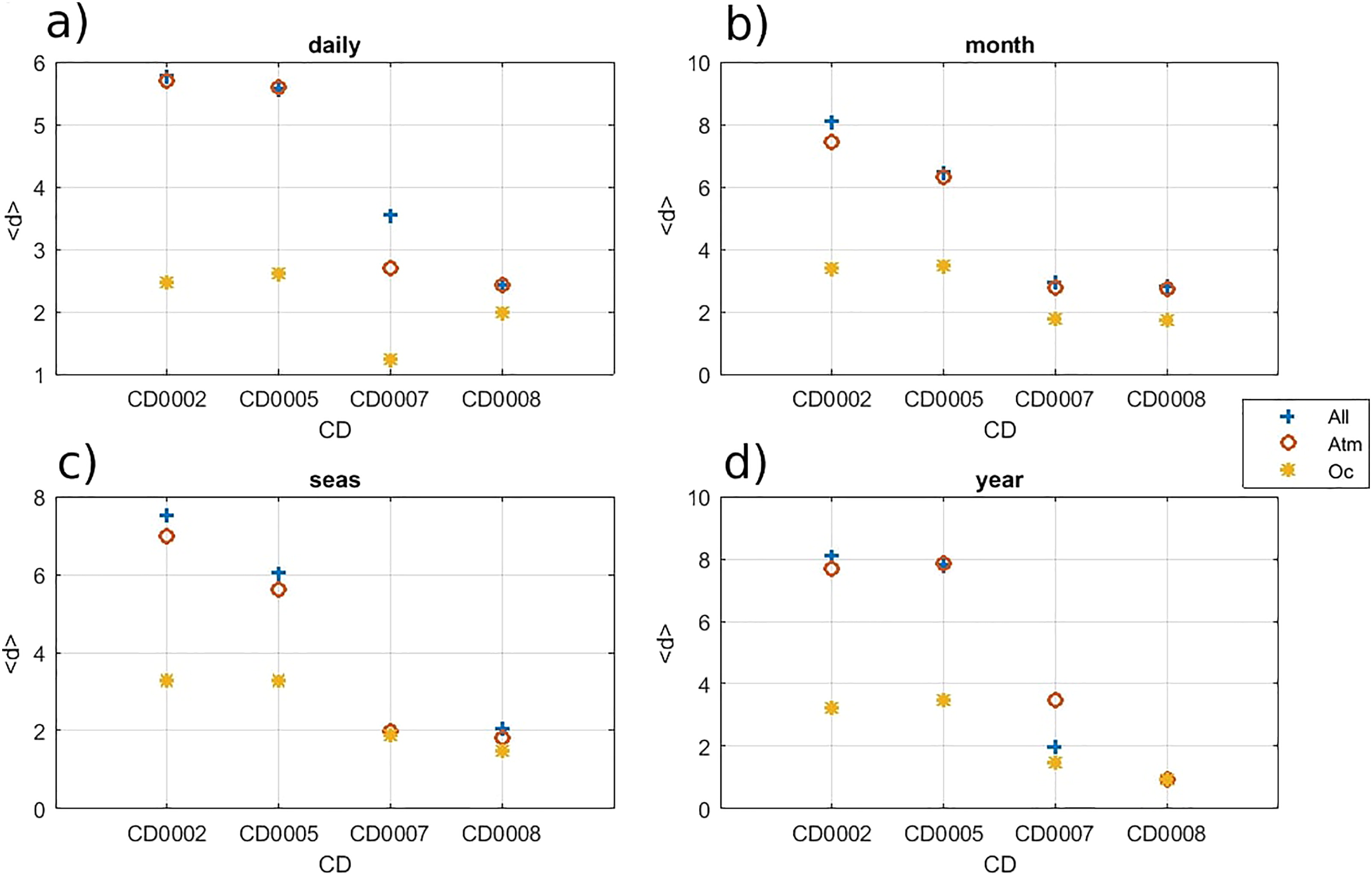
Fig. 5.
Attractor dimensions computed selecting all modes (blue crosses) atmospheric modes only (red circles), oceanic modes only (yellow stars). (a) daily, (b) monthly, (c) seasonal and (d) yearly data.
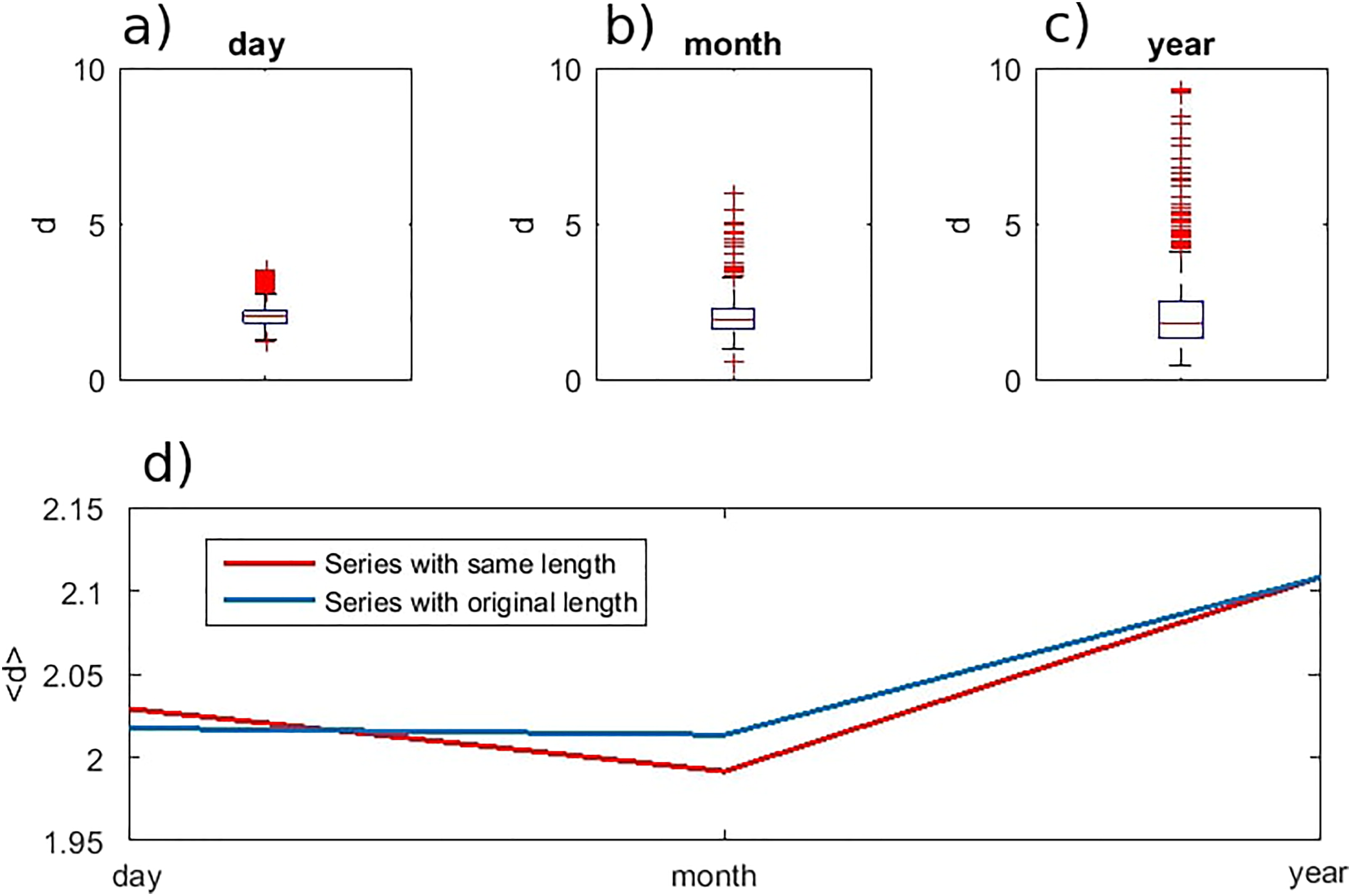
Fig. 6.
(a–c): boxplots of local dimensions d for NAO and Nino3 indices at different time scales. On each box, the central mark is the median, the edges of the box are the 25th and 75th percentiles, the whiskers extend to the most extreme data points not considered outliers, and outliers are plotted individually. (a) daily, (b) monthly and (c) yearly data. (d): average dimensions computed with the full length time-series (blue) and only 947 time steps (red).