
Fig. 1.
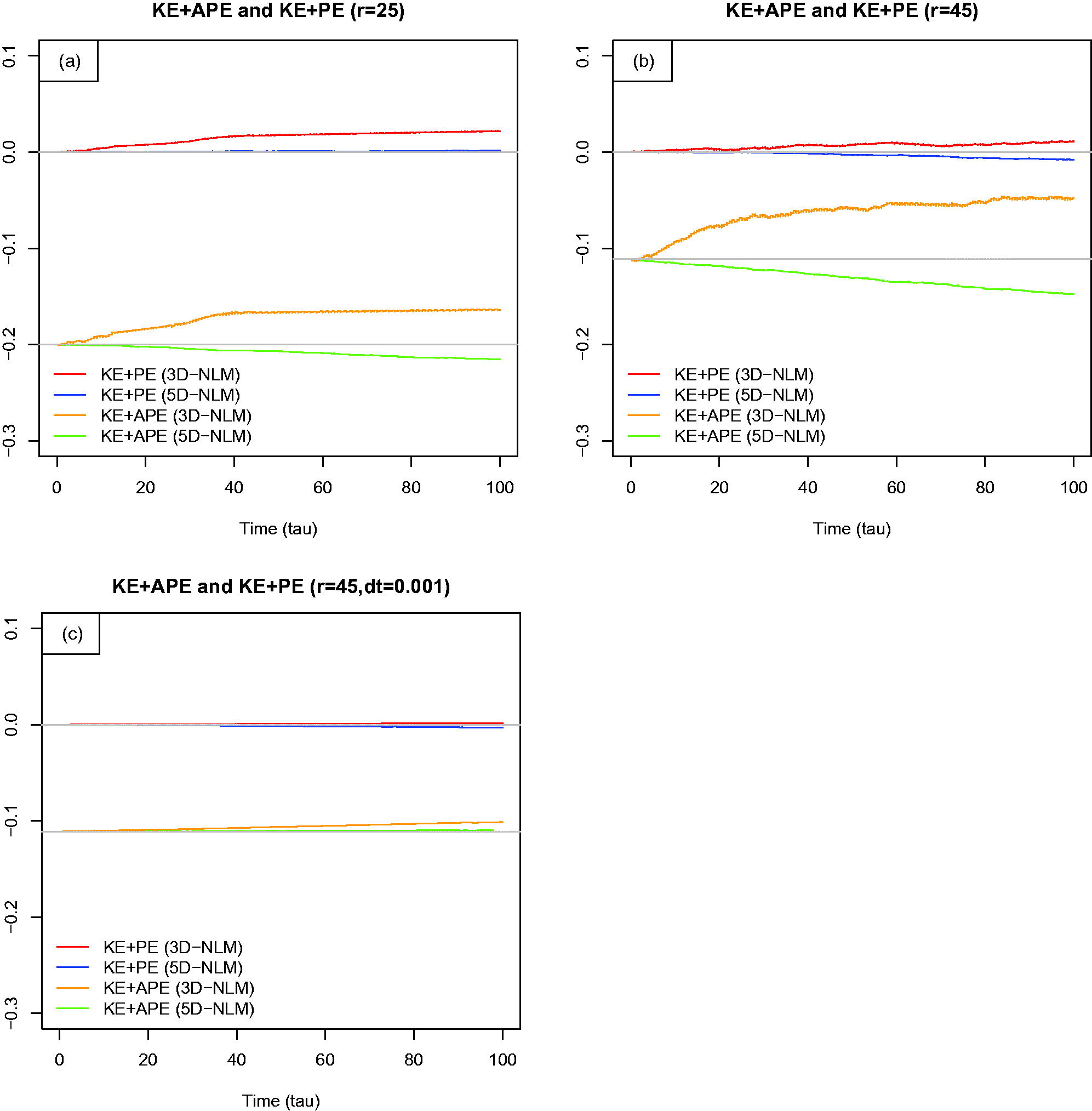
The time evolution of (KE + PE) and (KE + APE) from the 3D-NLM and 5D-NLM. Panels (a) and (b) are provided for r = 25 and r = 45, respectively. Results obtained from the 5D-NLM are presented in order to show the dependence of solutions on the spatial resolutions. In comparison with panel (b), panel (c) shows the dependence of solutions on the temporal resolution using Δτ = 0.0001. All of the fields are normalized using the constant Co .
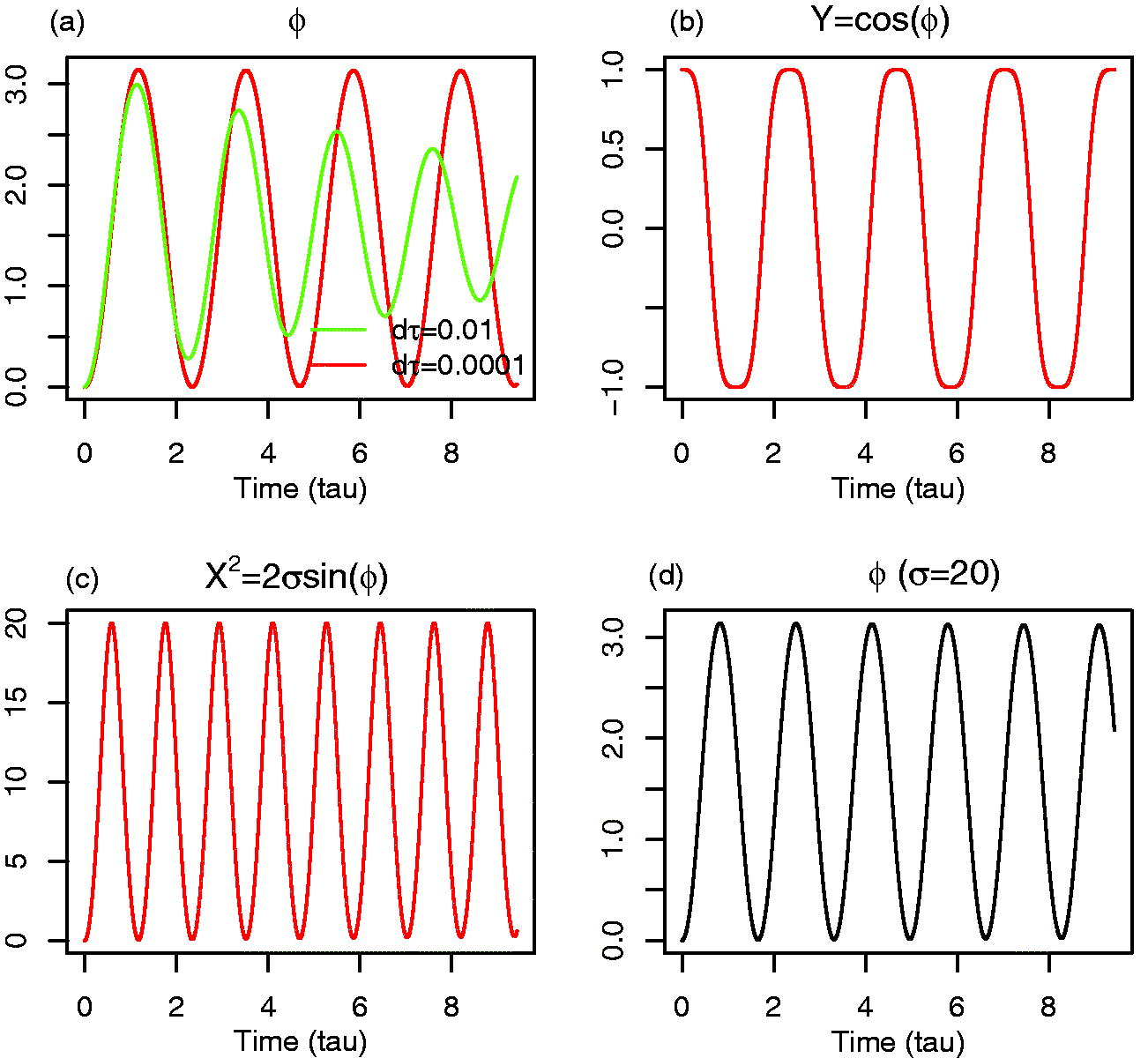
Fig. 2.
Closed-form solutions obtained from Equations (24a,b) using and the iterative method. (a) The phase function(ϕ) with (green) and (red) (Equation (24b)). (b) (Equation (24a)). (c) (Equation 18b). (d) The phase function using a different value of σ (=20).
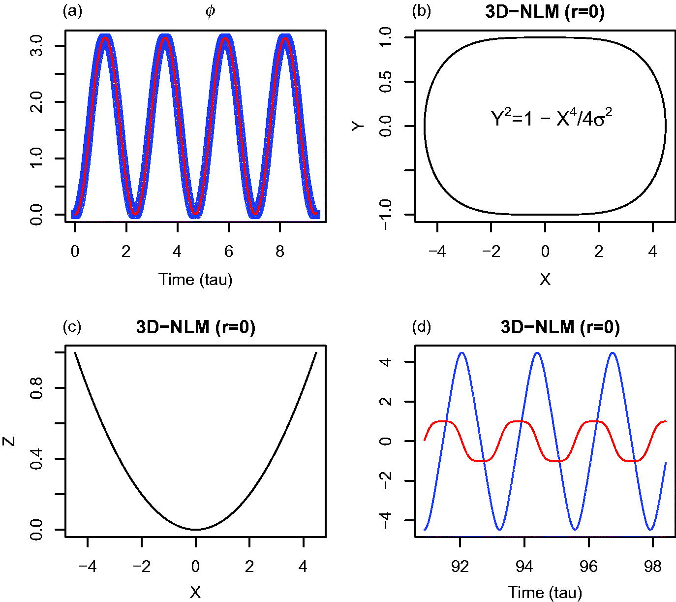
Fig. 3.
Numerical solutions obtained from the 3D-NLM (Equations (3)–(5)) using . (a) A comparison of the phase functions that are calculated from numerical solutions of the 3D-NLM (blue dot) and closed-form solutions of Equation (24a,b) (red). (b) X–Y plot. (c) X–Z plot. (d) The time evolution of X (blue) and Y (red).
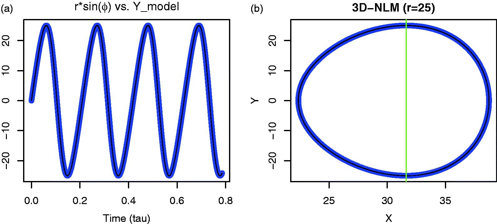
Fig. 4.
Closed-form solutions obtained from Equations (32c,d) using and and the iterative method. (a) A comparison of the closed-form solution (r*sin(ϕ)) from Equation (32a) and the numerical solution of Y from the 3D-NLM. (b) X–Y plot. Closed-form solutions are displayed using black lines and numerical solutions obtained from the 3D-NLM are shown with blue dots. The green line passes through the corresponding critical points at .
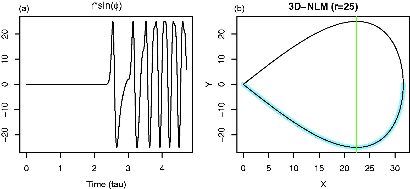
Fig. 5.
Closed-form solutions with Xo = 0 and the analytical solution of the homoclinic orbit. (a) The closed-form solution (r*sin(ϕ) of Equation (32a). (b) The X–Y plot for the closed-form solutions of Equation (32) (black) and the analytical solutions of the homoclinic orbit using Equation (34) (lightblue). The green line passes through the corresponding critical points at .
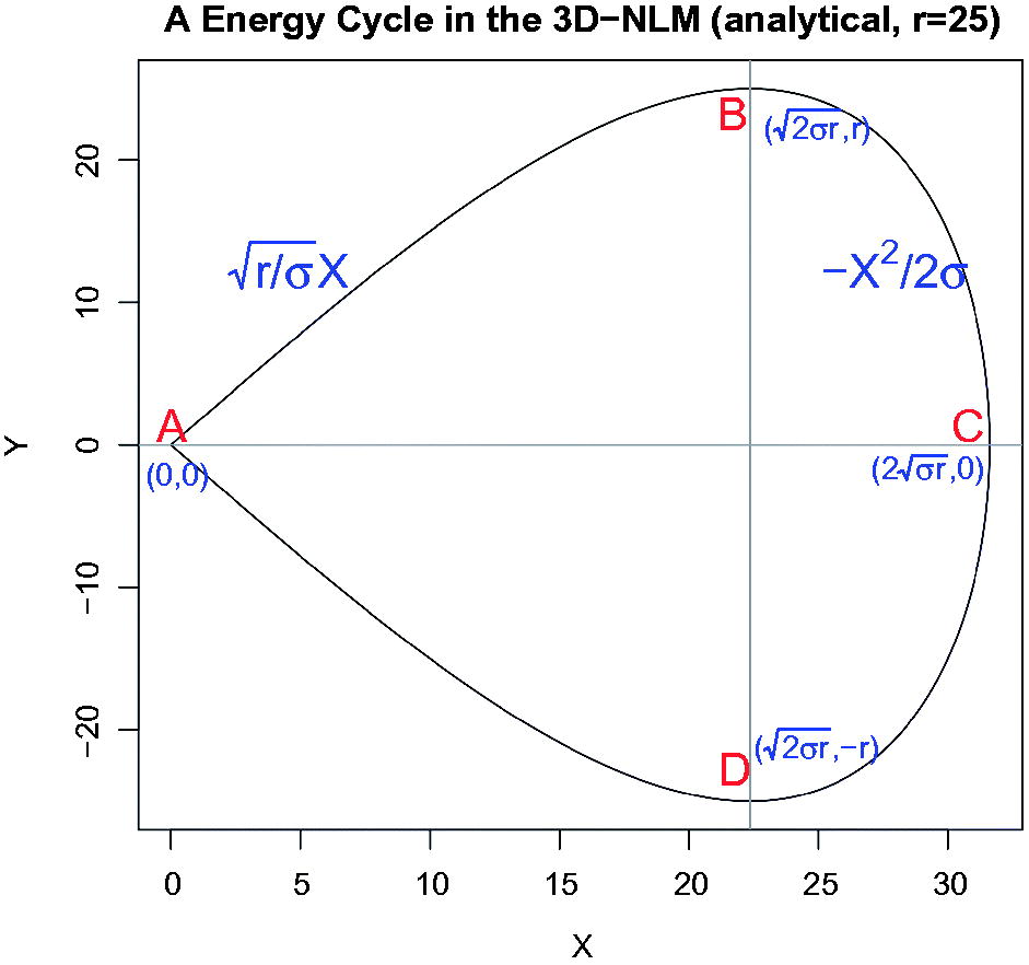
Fig. 6.
An energy cycle in the 3D non-dissipative Lorenz model (3D-NLM), as shown in the X–Y plot. The four points for the selected ICs are identified, as follows: A(X,Y) = (0,0), B = (), C = (), and D = (). (σ,r) = (10, 25). The energy cycle: (1) begins at the saddle point ; (2) goes through B, C, and D; and (3) returns near A. KE increases as APE decreases along the upper curve (Legs A–B and B–C), and KE decreases as APE increases along the lower curve (Legs C–D and D–A). From a perspective of potential energy partitioning, in Legs A–B and D–A where the linear force dominates, and in Legs B–C and C–D where the nonlinear restoring force dominates.
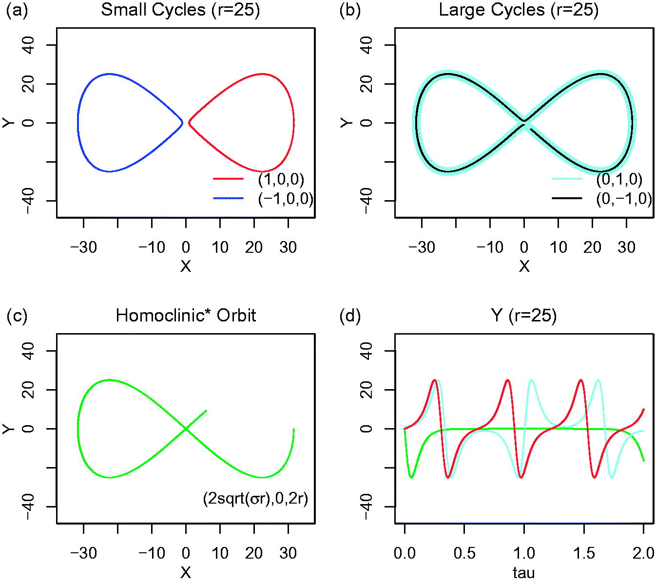
Fig. 7.
Three types of solutions associated with different ICs from the 3D-NLM (Equations (3)–(5)) with Δτ = 10−5 and τ = 4. (a) Oscillatory solutions with small cycles. (b) Oscillatory solutions with large cycles. (c) A numerical solution for the homoclinic orbit. (d) The time evolution of the simulated homoclinic orbit (green), and oscillatory solutions with a small cycle (red) and a large cycle (lightblue). Panels (c–d) indicate that the homoclinic trajectory begins at (X, Y, Z) = ( 0, 2r), approaches the origin, and remains near the saddle point for a much longer period of time as compared to the oscillatory solutions. Note that as a result of accumulated numerical error, the ‘simulated orbit’ travels around the saddle point, moves to the other side in panel (c), and is no longer the original homoclinic orbit.
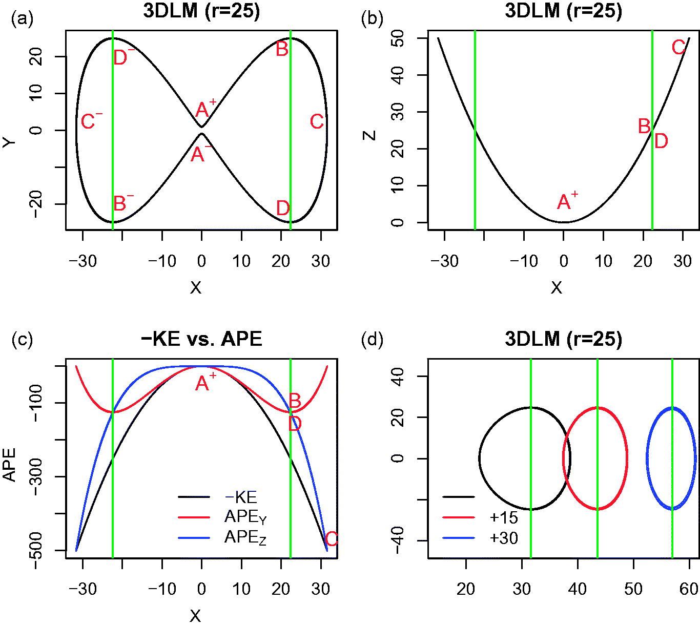
Fig. 8.
Solutions obtained from the 3D-NLM (Equations (3)–(5)). (a) X–Y plot. (b) X–Z plot. (c) X-APE plot. The black, red, and blue lines show normalized −KE, APEY, and APEZ, respectively. Green lines are plotted at where Y2 = Z2. (d) The X–Y plot using different initial conditions, (X, Y, Z) = (X0, 0, 0). The black, red, and blue curves represent results using , and , respectively. The three green lines pass through the corresponding critical points at (Xc, Yc) = .
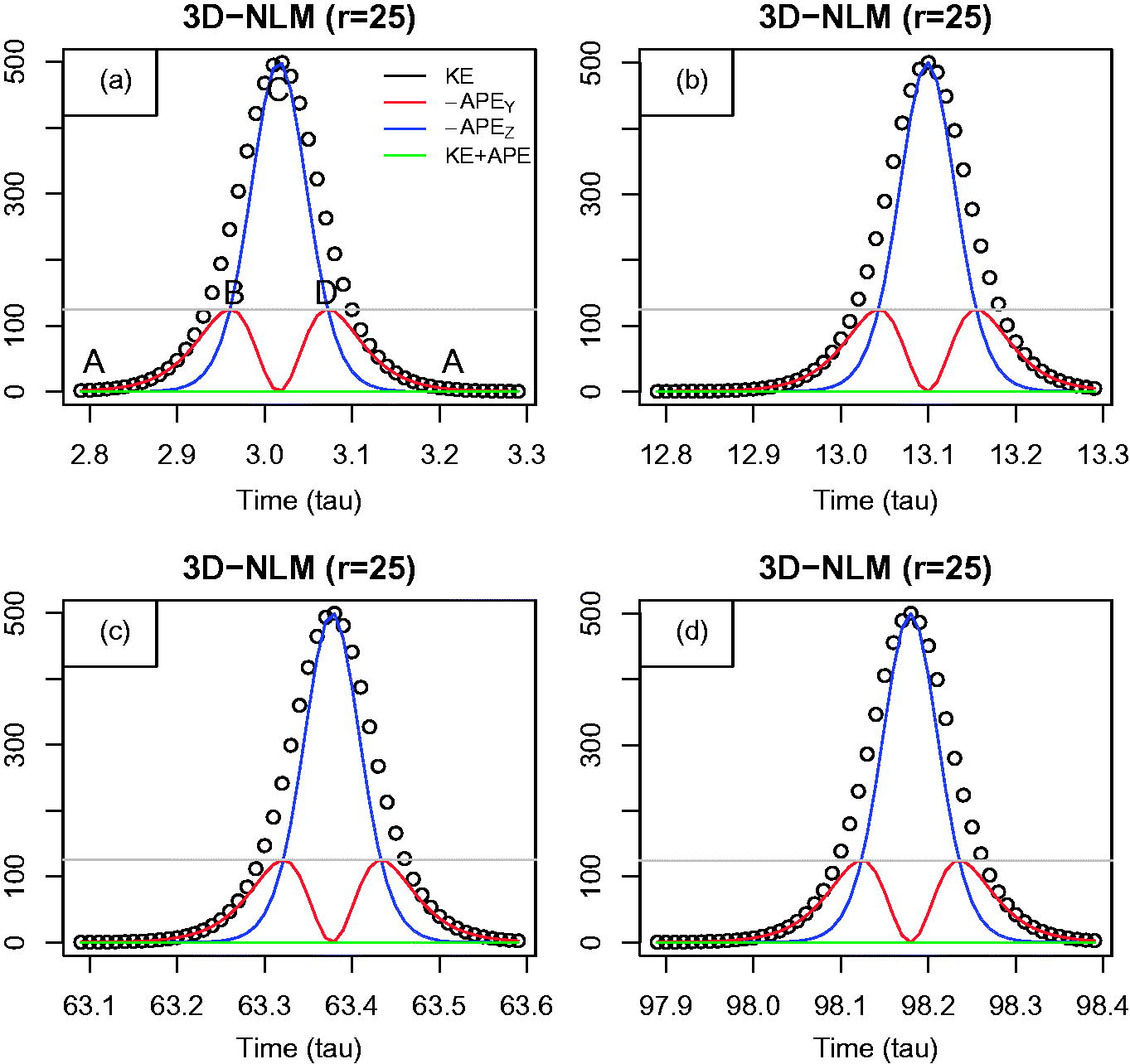
Fig. 9.
Time evolution for the KE and APE in the 3D-NLM (Equations (13)–(14)). Black open circles display KE. Red, blue, and green lines indicate −APEY, −APEZ, and KE + APE, respectively. All of the fields are normalized by Co. The gray line is plotted at a value of σr/2, which is equal to −APEY/Co and −APEZ /Co at X = Xt. These panels show that the solutions are oscillatory and periodic.
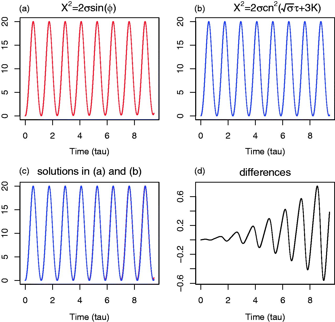
Fig. C1.
A comparison of the nonlinear oscillatory solutions using r = 0 in Equations (18b) and (C9), expressed using an elementary trigonometric function and an elliptic function, respectively. (a) The solution of Equation (18b) in red. (b) The solution of Equation (C9) in blue. (c) Both of the solutions in (a) and (b). (d) Differences of the two solutions.