
Introduction
1.
It has been 50 years since Lorenz published his breakthrough modeling study (Lorenz, 1963) that changed our views on the predictability of weather and climate (Solomon et al., 2007). The model has been extensively investigated by researchers in various fields including earth science, engineering, mathematics, philosophy, and physics (Gleick, 1987; Sprott, 2003; Jordan and Smith, 2007; Anthes, 2011; Hirsch et al., 2013; Strogatz, 2015). Lorenz’s model with three Fourier modes, which represents the solution to the 2-D Rayleigh–Benard equation (Saltzman, 1962; Lorenz, 1963), is known as the three-dimensional Lorenz model (3DLM). In this paper, we use 3D-NLM to refer to the non-dissipative version of the model that is introduced later in the text.
The scientific community agrees that weather is chaotic, with a finite predictability, and that the source of chaos is nonlinearity. Since the degree of nonlinearity is finite within the 3DLM, the impact of increased nonlinearity on system solutions and/or their stability has been studied using generalized LMs with additional Fourier modes (Curry, 1978; Curry et al., 1984; Howard and Krishnamurti, 1986; Hermiz et al., 1995; Thiffeault and Horton, 1996; Musielak et al., 2005; Roy and Musielak, 2007a). As compared to the 3DLM, some of the generalized LMs have suggested larger Rayleigh number values (or heating parameters) for the onset of chaos, while others have indicated smaller values. This discrepancy may be attributed to different mode truncations (Curry et al., 1984; Thiffeault and Horton, 1996; Roy and Musielak, 2007a,b,c; Shen, 2014, 2015, 2016) that lead to different degrees of nonlinearity and different systems whose energy may or may not be conserved (Roy and Musielak, 2007a).
Among studies using generalized LMs, the pioneering study of Prof. Curry (Curry et al., 1984) suggested that chaotic responses disappeared when sufficient modes are included. Recent studies by Prof. Musielak and co-authors (Musielak et al., 2005; Roy and Musielak, 2007a,b,c) have examined the transition to chaos and the fractal dimensions of generalized LMs, and have emphasized the importance of proper mode truncation in energy conservation. More recent studies (Shen, 2014, 2015, 2016) have discussed the importance of proper Fourier mode selection in extending the nonlinear feedback loop of the 3DLM. The feedback loop, which consists of the two nonlinear terms of the 3DLM, includes a pair of down-scale and up-scale transfer processes associated with the Jacobian function of the partial differential equation, discussed in Section 2. As previously suggested, the original feedback loop may help stabilize the solution for 1 < r < 24.74 within the 3DLM. The extended nonlinear feedback loop in high-dimensional LMs can provide negative nonlinear feedback that produces non-trivial stable critical points when r < 42.9 within a five-dimensional LM and when r < 116.9 within a seven-dimensional LM. Based on the above, it has been hypothesized that a system’s stability can be improved further with additional modes that can provide negative nonlinear feedback. While the importance of an increased degree of nonlinearity with more Fourier modes has been discussed in recent studies, the competing role of the nonlinear terms with the linear (heating) term and/or dissipative terms deserves to be examined in order to ascertain the conditions under which nonlinear processes may lead to stable or chaotic solutions.
Roupas (2012) and others have indicated that the 3DLM in the dissipative limit, which is referred to as the 3D-NLM, contains two conserved quantities that represent the conservation of () and (), respectively. Here, , and are the domain-averaged kinetic energy, potential energy, and available potential energy, respectively. These two quantities, () and (), are related to the Nambu Hamiltonians (Nambu, 1973; Nevir and Blender, 1994; Floratos, 2012; Roupas, 2012; Blender and Lucarini, 2013). As a result of conservation properties, the collective impact of the nonlinear feedback loop and the linear (heating) term may effectively act as a “restoring” force. The simplicity of the 3D-NLM enables an examination of how the nonlinear feedback loop and the linear (heating) term work together to produce oscillatory solutions (in the phase space). In this work, we address this issue in conjunction with how the available potential energy is partitioned amongst two different Fourier modes, Y and Z, where Z is included in order to enable the nonlinear feedback loop.
The paper is organized as follows: In Section 2, we present the governing equations and the 3D-NLM, introduce the nonlinear feedback loop, and derive the energy conservation laws. In Section 3, we illustrate the role of the nonlinear feedback loop (with r = 0) in acting as a restoring force. With inclusion of the heating term, as well as the nonlinear feedback loop, we present a linear stability analysis for the three critical points and then discuss three types of solutions using analytical and numerical methods. The solutions include two types of oscillatory solutions and the so-called homoclinic orbit (Sprott, 2003; Jordan and Smith, 2007). An energy cycle with four regimes is analyzed based on the tendency of and the partition of at different scales (i.e. either Y or Z). Concluding remarks are provided at the end. Appendix A discusses the derivation of the 3D-NLM, and Appendix B illustrates the relationship between the nonlinear feedback loop and the nonlinear restoring force. Appendix C presents a closed-form solution to the system with r = 0 using elliptic functions (Davis, 1960). Appendix D discusses the equations and initial conditions that are used to obtain the solution of the homoclinic orbit.
Governing equations and the non-dissipative Lorenz model
2.
The following governing equations for a 2D (x, z), Boussinesq flow are introduced in order to derive the non-dissipative Lorenz model (3D-NLM) and to calculate its kinetic and potential energy:
where ψ is the streamfunction that yields and that represent the horizontal and vertical velocity perturbations, respectively, and θ is the temperature perturbation. represents the temperature difference between the bottom and top boundaries. The constants, g, α, ν, and κ denote the acceleration of gravity, the coefficient of thermal expansion, the kinematic viscosity, and the thermal diffusivity, respectively. The Jacobian of two arbitrary functions is defined as . The crossout symbol indicates the negligence of a term in the dissipationless limit. Equations (1) and (2), with the dissipative terms, were first used in Saltzman (1962) and Lorenz (1963).The non-dissipative Lorenz model (3D-NLM) is written as:
Here, (X, Y, Z) represent the amplitude of the Fourier modes. is the dimensionless time. a is the ratio of the vertical scale of the convection cell to its horizontal scale. H is the domain height, and represents the domain width. is the Prandtl number, and is the normalized Rayleigh number or the heating parameter. is the Rayleigh number, , and is the critical value for the free-slip Rayleigh–Benard problem, . The ‘forcing’ terms on the right-hand side of Equations (4) and (5) are referred to as the linear force, or the heating term (rX), and the nonlinear force terms (–XZ and XY). Note that as a result of scale selection in the original Lorenz model, the appearance of σY comes from , which represents a buoyancy term (Hilborn, 2000), and is not associated with the dissipative terms. Appendix A provides detailed derivations.
The 3D-NLM is integrated forward in time using the fourth-order Runge–Kutta scheme. Without a loss of generality, only three different values of the normalized Rayleigh number, r (r = 0, r = 25, and r = 45) are used, while keeping other parameters, including σ = 10 and , constant. A dimensionless time interval () of 0.01 is used and the total number of time steps is 10,000, giving a total dimensionless time (τ) of 100. A smaller is used to improve accuracy. In this study, unless stated otherwise, the initial conditions (ICs) are as follows:
These settings were used in order to examine the stability of the 5DLM and 6DLM in Shen (2014, 2015), who also discussed the dependence of the solution on different r and σ. To illustrate the unique features of solutions, a very small time step and/or different ICs are used, including , , and . The first IC is used for showing solutions with a small cycle, and the second is used for discussing solutions with a large cycle. The third IC is used to perform a numerical simulation for the homoclinic orbit (Sprott, 2003; Jordan and Smith, 2007). In this study, we use a tiny ϵ in Fig. 5 and ϵ = 1 in Fig. 7.
The nonlinear feedback loop and energy conservation laws
2.1.
Nonlinear terms in the 3D-NLM (and 3DLM) have been shown to result from the Jacobian term, , in Equation (2). The nonlinear interaction of two wave modes via the Jacobian term can generate or impact a third wave mode through a downscale (or upscale) transfer process. The subsequent upscale (or downscale) transfer process associated with the third wave mode can provide feedback to the incipient wave mode(s). As illustrated in Shen (2014), XY and –XZ, respectively, represent the downscale and upscale transfer processes that form a nonlinear feedback loop. When new modes are properly included, the feedback loop can be extended. In the following subsections, we discuss the role of the 3D-NLM nonlinear feedback loop in the energy conservation and partition of available potential energy, which, in turn, helps produce oscillatory solutions.
The domain-averaged kinetic energy (), the potential energy (), and the available potential energy () are defined as follows (Thiffeault and Horton, 1996; Blender and Lucarini, 2013; Shen, 2014, 2015):
Through straightforward derivations, we obtain the following:
where . is non-positive (i.e. ), since any perturbation reduces the energy transformable to .Equations (10) and (11) lead to:
while Equations (10) and (12) yield:With Equations (3)–(5), the time derivative for both Equations (13) and (14) is zero, so these two equations describe energy conservation. Both C1 and C2 are constants and are determined by the initial conditions. Thus, if we express Z and Y2 as functions of X, they are single valued. To facilitate our discussions, the contribution to APE from an individual mode is defined as , where I = Y or Z; therefore, . Note that Equations (13) and (14) are related to the two Nambu Hamiltonians, and (Nambu, 1973; Nevir and Blender, 1994; Floratos, 2012; Roupas, 2012; Blender and Lucarini, 2013).
From the initial conditions in Equation (6), we have and , the latter of which is –0.2 for r = 25 and –0.11 for r = 45. Figure 1 provides the time evolution of the conserved quantities: () and () in Equations (13) and (14) from the 3D-NLM. At a larger r (e.g. r = 45), a finer is required to improve the numerical accuracy of simulated total energy (Fig. 1c). In this study, to facilitate discussions and unless stated otherwise, either C1 or C2 is assumed to be zero.
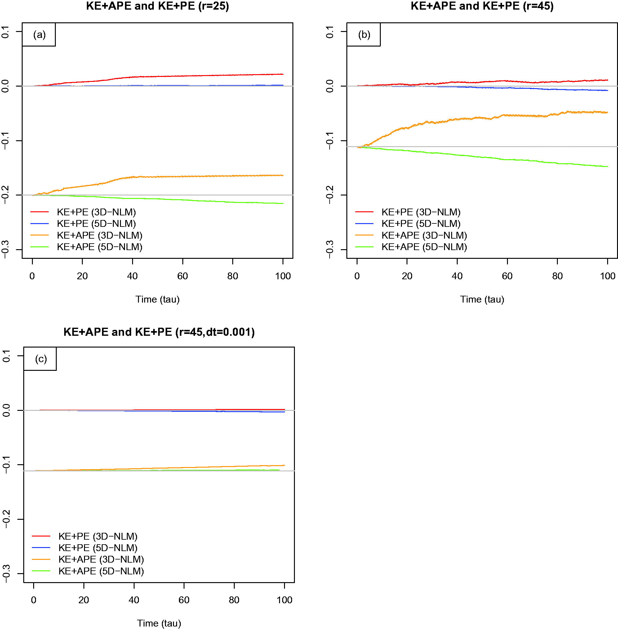
Fig. 1.
The time evolution of (KE + PE) and (KE + APE) from the 3D-NLM and 5D-NLM. Panels (a) and (b) are provided for r = 25 and r = 45, respectively. Results obtained from the 5D-NLM are presented in order to show the dependence of solutions on the spatial resolutions. In comparison with panel (b), panel (c) shows the dependence of solutions on the temporal resolution using Δτ = 0.0001. All of the fields are normalized using the constant Co .
Discussions
3.
In this section, we discuss the competing role of the nonlinear terms and the linear forcing term in the transient solutions and the energy cycle of the 3D-NLM. From Equations (3), (4), and (13), we obtain
andThe three terms on the right-hand side of Equation (15b) represent the impact of nonlinearity, the linear (heating) force, and the initial conditions, respectively. Their competing impacts (i.e. their differences) determine the sign of M2, and thus, the characteristics of the solution. Based on the relative magnitude of the initial state that may lead to or >0, two types of solutions can be identified (Roupas, 2012). Please note that Equation (15) is a special case of Duffing Equation when and is called the double-well potential system when . Some exact solutions to the Duffing equation or double-well potential system can be found in other studies (Drazin, 1992; Jordan and Smith, 2007; Elias-Zuniga, 2013; Starossek, 2015). In this study, we focus on the role of nonlinear feedback loop in producing the oscillatory solutions as well as the homoclinic orbit and on the physical interpretation of the solutions, including the mechanism for diverged trajectories, as discussed below. Therefore, we study the case with by using in Section 3.2 and in Section 3.3, where Xo is the initial value of X. To understand the role of the nonlinear terms (i.e. the nonlinear feedback loop), we begin discussions by solving the solution to the equation that contains no nonlinear terms.
Solutions of the linear system without the nonlinear feedback loop
3.1.
By assuming no nonlinear terms, we can begin with two equations: and and only one conservation law, as follows:
This linear case yields , and Equation (15) becomes A local analysis suggests that the origin, the only critical point in the linear system, is a saddle point. After straightforward derivations, the solution is:
where X1 and X2 are constant coefficients. The origin is a saddle point, and the trajectory is hyperbolic with solutions exhibiting exponential growth and decay. The initial condition, which determines , can help select the proper mode(s). For example, only provides the growing mode with , while leads to the decaying mode with . The former and latter display the properties of unstable and stable manifolds, respectively (Ide et al., 2002). For the nonlinear case, a ‘current’ state (i.e. ICs) may vary with time. Therefore, either mode may appear at different stages. For example, as shown with the homoclinic orbit in Section 3.3, a trajectory with an initial point of may approach the origin at a decay rate of , while a trajectory beginning near the origin may depart at a growth rate of . Based on Equations (16) and (17), although the time change of () remains zero, the produced using only the linear (heating) force has no upper limit. Such an outcome could violate the linear assumption, and, thus, nonlinearity should be included.Nonlinear solutions and the nonlinear restoring force for r = 0
3.2.
Here, we examine the impact of nonlinear terms using a special case with r = 0 and , leading to . Thus, Equation (15) and its solution are written as follows:
In Appendix B, we show that the cubic term (X3) in Equation (18a) is derived from the nonlinear feedback loop (–XZ and XY). The solution in Equations (18b) and (18c) is periodic and it has time varying frequencies. More importantly, as discussed later, when the approach is applied to the system with , we can also obtain periodic and bounded solutions, which is different from the unbounded solution of the linear system in Equation (17). Thus, we suggest that the nonlinear feedback loop (i.e. the cubic term) acts as a restoring force. Solutions for other components (Y and Z) can be obtained as follows.
As compared to the case with in Equations (13) and (14), the energy conservation laws obtained using r = 0 are:
which, in turn, lead to:Since X2 is defined in Equation (18b), solutions for Y and Z can be obtained as follows:
where the phase function, in Equation (18c), can also be displayed as:To illustrate the solution’s characteristics, Equations (22a) and (23) are solved using the following iterative method:
where N is the number of iterations. Over a period of time, an initial guess for the phase function is given as . We insert the first phase function, , into Equation (24a) to obtain Y0. We then calculate the next phase function, , using Y0 and Equation (24b). The integral in Equation (24b) is calculated using the trapezoidal rule. We then repeat the above calculations N times. Numerical results using N = 100 are provided in Fig. 2. The phase function (Fig. 2a) oscillates with time and varies between 0 and π, consistent with Equation (18b) as a result of . Therefore, the solution to Equation (18a) is oscillatory instead of growing or decaying exponentially (as shown in Figs. 2b and 2c). The nonlinear term in Equation (18a) may be viewed as a nonlinear restoring force. Such a suggestion is consistent with the view (Shen, 2014) that the pair of nonlinear terms (–XZ and XY), leading to the nonlinear term (), can form a nonlinear feedback loop within the 3DLM. Appendix B provides a brief summary. When σ = 10 is replaced by σ = 20, an oscillatory solution with a different period is obtained, as shown in Fig. 2d. As a result of the simple method for integral calculation, a fine may be required in order to obtain accurate solutions, as indicated by the red and green lines for the results obtained using and 0.01, respectively (Fig. 2a).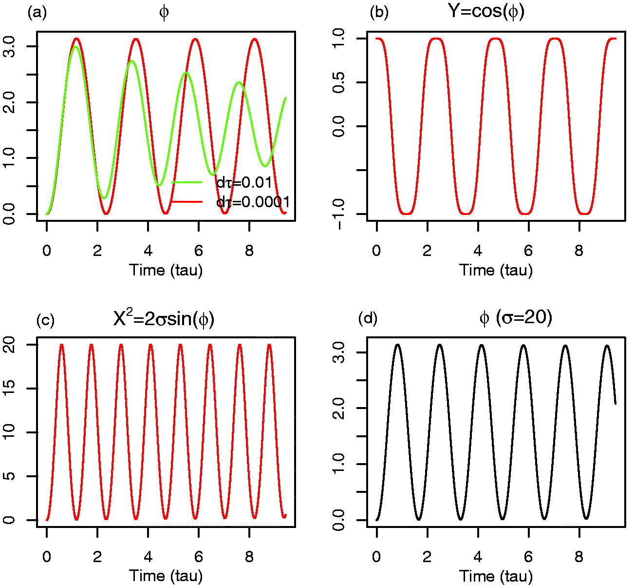
Fig. 2.
Closed-form solutions obtained from Equations (24a,b) using and the iterative method. (a) The phase function(ϕ) with (green) and (red) (Equation (24b)). (b) (Equation (24a)). (c) (Equation 18b). (d) The phase function using a different value of σ (=20).
To verify the integral form of the solutions in Equations (24a) and (24b), the numerical solutions of the 3D-NLM using r = 0 (Equations (3)–(5)) are provided in Fig. 3. In panel (a), the blue ‘dot’ indicates the initial temporal evolution of the phase function that is calculated by performing a time integration of X using Equation (18c), where X is obtained from the 3D-NLM; and the red line indicates the phase function calculated using Equations (24a) and (24b). Both are in good agreement. The simulated trajectories in the X–Y and X–Z sections are elliptic and parabolic (Figs. 3b and 3c), respectively, consistent with the analytical relationships in Equations (21) and (19), respectively. Figure 3d provides the time evolution of oscillatory Y (red) and X (blue), consistent with the results provided in Figs. 2b and 2c, respectively. As indicated in Appendix C, the oscillatory characteristics of the solution can also be illustrated using elliptic functions.
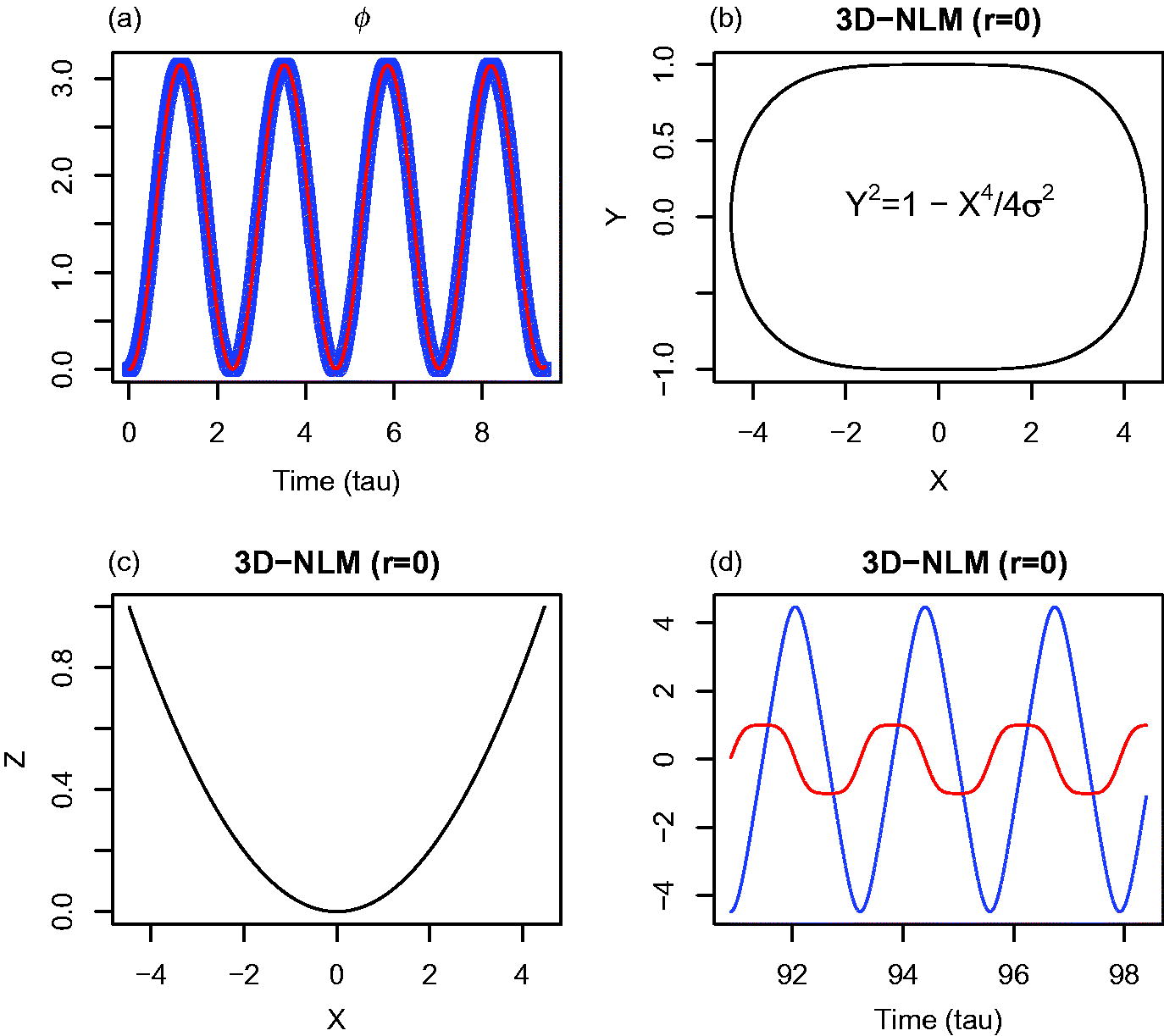
Fig. 3.
Numerical solutions obtained from the 3D-NLM (Equations (3)–(5)) using . (a) A comparison of the phase functions that are calculated from numerical solutions of the 3D-NLM (blue dot) and closed-form solutions of Equation (24a,b) (red). (b) X–Y plot. (c) X–Z plot. (d) The time evolution of X (blue) and Y (red).
Closed form solutions near a non-trivial critical point for
3.3.
In the previous sections, we used Equation (15) to illustrate the individual impact of the linear (heating) force and the nonlinear feedback loop using cases with M2 < 0 and , respectively, neither of which changes the sign during the integration. Here, using the initial condition and , we consider a more general case with , whose sign may vary during the time integration depending on the relative magnitude of the nonlinearity and the linear (heating) force. M2 has two zeros at , where is defined as . These are called turning points. Based on an analysis using the WKB approximation (Bender and Orszag, 1978), there appears to be a growing or decaying solution for and an oscillatory (wave-like) solution for . The former is largely impacted by the linear (heating) force while the latter is impacted by the nonlinear restoring force. Additional analyses are provided below.
To understand the stability of solutions, below, we present a local analysis by linearizing the system with respect to a non-trivial critical point. Using Equations (3)–(5), we first solve for the non-trivial critical point, which is . Here, Xc can be any constant and is selected as the value of X at the turning point of Equation (15) using the justification presented below. From Equations (3) and (15), the 3D-NLM system can be written as:
The two equations, with an initial condition of (X, Y) = , lead to three critical points, (Xc, Yc) at (0, 0) and . Note that the non-trivial critical points are determined by the condition M = 0, which defines the turning points in Equation (15). Therefore, we have Xc = Xt.
Next, each of the total fields is decomposed into its basic part and perturbation, as follows:
where V indicates the total fields (X, Y, Z), Vc represents the basic state obtained from the solution of the critical point, and is a perturbation that measures the departure from the critical point. Using the above equation, the linearized system corresponding to the nonlinear system from Equations (3)–(5) is: where and the matrix A that is evaluated at the non-trivial critical point is written as:The above system with Equations (28)–(29) yields eigenvalues of 0 and , suggesting that the non-trivial critical point () for the linearized system is a stable node as a center. The other non-trivial critical point (−) shares the same features. One important feature is the dependence of the solution’s period () on the initial condition (Xo). Next, to illustrate its periodicity, we present a closed form solution for the nonlinear system.
Equations (13)–(14), with the initial conditions (X, Y, Z) = (), lead to the following two equations:
Using the same procedures as those provided in Section 3.2 (for r = 0), the following closed-form solutions (for are obtained:
Equations (32c) and (32d) are iteratively computed in order to determine the value of that is used to calculate the solutions of X, Y, and Z. Note that because , Equations (32a) and (32c) lead to:
Since , X2 is always positive in Equation (32c). Without a loss of generality, is first discussed, yielding a minimum of and a maximum of . In a similar manner, given an initial condition of , X has a maximum of and a minimum of . Note that the average of and is equal to , which is equal to .
Applying the initial conditions that yield (), Fig. 4 shows the closed form solutions obtained using Equation (32), as well as numerical solutions of the 3D-NLM obtained using Equations (3)–(5). The results are in good agreement. For any positive Xo, a trajectory beginning with is a closed curve. An oscillatory (closed) trajectory associated with a center is orbitally stable (Jordan and Smith, 2007). In Section 3.4, the time varying energy cycle in Equation (32) will be analyzed. Next, we discuss the solutions in (32) for the special case of Xo = 0.

Fig. 4.
Closed-form solutions obtained from Equations (32c,d) using and and the iterative method. (a) A comparison of the closed-form solution (r*sin(ϕ)) from Equation (32a) and the numerical solution of Y from the 3D-NLM. (b) X–Y plot. Closed-form solutions are displayed using black lines and numerical solutions obtained from the 3D-NLM are shown with blue dots. The green line passes through the corresponding critical points at .
When considering a homoclinic solution that begins with and ends at the saddle point, initial conditions of are required. At the saddle point, the time derivatives of the 3D-NLM in Equations (3)–(5) are zero. Therefore, numerically, only zero solutions for X, Y, and Z are possible. Obtaining a non-trivial solution can be attempted by initially adding a small perturbation (i.e. ) and then performing numerical integrations. A similar approach can be applied in Equation (32) to obtain an approximate solution. Here, we provide an initial guess for , over a target period in Equation (32d). We then calculate X using Equation (32c) and using Equation (32d) through iterations. Figure 5 displays the solutions determined using Equation (32). The time evolution of Y is provided in Fig. 5a and suggests that Y increases slowly with time, reaches a maximum at , and then decreases with time to its minimum. The X–Y plot in Fig. 5b appears reasonable and is later compared to the analytical solution. In Fig. 5a, the evolution seems ‘periodic’ but displays some irregularities that are different from those obtained using . This case is further analyzed using the following analytical solution, as well as the numerical solutions in Section 3.5.
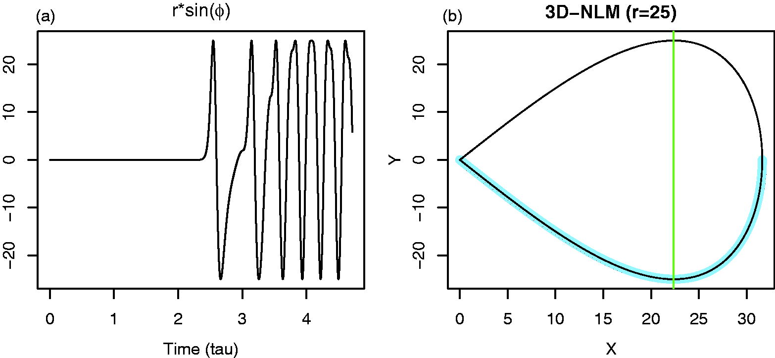
Fig. 5.
Closed-form solutions with Xo = 0 and the analytical solution of the homoclinic orbit. (a) The closed-form solution (r*sin(ϕ) of Equation (32a). (b) The X–Y plot for the closed-form solutions of Equation (32) (black) and the analytical solutions of the homoclinic orbit using Equation (34) (lightblue). The green line passes through the corresponding critical points at .
From Equation (D3) of Appendix D, the ‘second’ half of the homoclinic orbital solution (e.g. the lower part of the orbit in Fig. 5b) can be obtained as follows:
When , the above solution approaches the origin. Note that a special point on the solution trajectory is . Therefore, the ‘second’ half of the solution in Equation (34) describes the trajectory that begins at and that moves forward in time toward the origin, as shown in light blue in Fig. 5b. The special point provides an alternative IC for the numerical integration of the 3D-NLM required to simulate (qualitatively) the homoclinic orbit, discussed with numerical results later. When , and , yielding . These features are the same as those for the linear (stable) solution with a heating term, as outlined in Section 3.1. As the system is invariant under and (Strogatz, 2015), the solution ( in backward time, which represents the ‘first’ half of the solution, displays the trajectory that begins at the origin and then moves to the point (e.g. the upper part of the orbit in Fig. 5b). The total solution that consists of the first and second half connects the stable and unstable manifolds of the saddle point and is called the homoclinic orbit. Since the trajectory ‘takes forever’ to reach the saddle point (as ), it is, therefore, not a periodic solution. As a result, the ‘periodicity’ of closed-form solutions with Xo = 0, as provided in Fig. 5, is spurious, suggesting a numerical error. Unique features of the homoclinic orbit within the analytical solution, as well as the closed-form solution, will be further explored using numerical solutions below.
An energy cycle of solutions with
3.4.
Here, we analyze the time evolution of energy along the homoclinic orbit and apply it to nearby trajectories with a small energy cycle. In Equation (D3), leads to , which yields a maximum of X () at Y = 0, denoted by Ym = 0. Taking the partial derivative of Equation (D3) with respect to X indicates that Y has extrema when . At , Z = r, and from Equations (13) and (14), respectively, and, thus, = , in other words equal contributions to from the Y and Z modes. Furthermore, Equation (D3) suggests that Y2 initially increases in association with the increase in X2 but later decreases in association with an increase in X4. The former is consistent with the linear case in Equation (16), while the latter is consistent with the simplified nonlinear case in Equations (19) and (20). The distribution of Y as a function of X Equation ((D3)), with the aforementioned four points, is provided in Fig. 6. The energy cycle: (1) begins at point A; (2) goes through B, C, and D; and (3) returns back to A. The segment from point P to point Q is designated as Leg P–Q, where P and Q are either one of the following: , , or . Point A is a saddle point as discussed in Section 3.1, , and . The energy cycle is referred to as a small (energy) cycle. From a perspective of potential energy partitioning, the linear force dominates in Legs A–B and D–A where , while the nonlinear restoring force dominates, in Legs B–C and C–D where . This also illustrates the importance of the inclusion of the Z mode and thus the nonlinear terms. Here, it should be noted that the homoclinic orbit is not periodic, and that a small energy cycle may appear within the oscillatory trajectories that move close to, but do not pass through, the saddle point. In the discussion provided in the next section, the analysis discussed above is inter-compared to the numerical solutions obtained from the 3D-NLM.
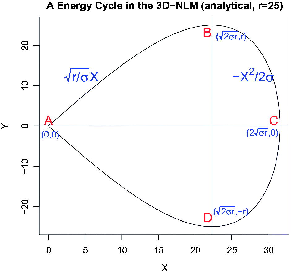
Fig. 6.
An energy cycle in the 3D non-dissipative Lorenz model (3D-NLM), as shown in the X–Y plot. The four points for the selected ICs are identified, as follows: A(X,Y) = (0,0), B = (), C = (), and D = (). (σ,r) = (10, 25). The energy cycle: (1) begins at the saddle point ; (2) goes through B, C, and D; and (3) returns near A. KE increases as APE decreases along the upper curve (Legs A–B and B–C), and KE decreases as APE increases along the lower curve (Legs C–D and D–A). From a perspective of potential energy partitioning, in Legs A–B and D–A where the linear force dominates, and in Legs B–C and C–D where the nonlinear restoring force dominates.
Numerical solutions with
3.5.
In this section, we first discuss the numerical solutions with small cycles that were analyzed in the previous section, and then present the numerical solutions with large cycles that enclose three critical points. The former are obtained using ICs of , while the latter are simulated with ICs of . Since the features of solutions (e.g. homoclinic orbits) require a high level of numerical accuracy, for Fig. 7, we perform numerical integrations using a very small time step of but for a shorter period of time (τ = 4). Figure 7a displays oscillatory solutions with small cycles, each of which moves around one of the non-trivial critical points. Figure 7b displays the two oscillatory solutions with a large cycle, moving around all three critical points. The two solutions share the same orbit. The numerical result of the ‘homoclinic orbit’ is shown in Fig. 7c. Figure 7d shows the evolution of these solutions. While the evolution of energy described by the small or large (energy) cycle will be analyzed later, we first discuss the results of ‘homoclinic orbit’.
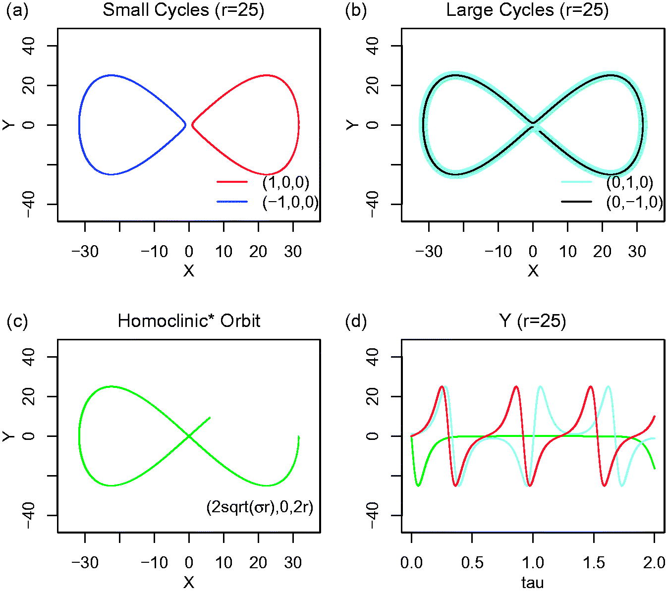
Fig. 7.
Three types of solutions associated with different ICs from the 3D-NLM (Equations (3)–(5)) with Δτ = 10−5 and τ = 4. (a) Oscillatory solutions with small cycles. (b) Oscillatory solutions with large cycles. (c) A numerical solution for the homoclinic orbit. (d) The time evolution of the simulated homoclinic orbit (green), and oscillatory solutions with a small cycle (red) and a large cycle (lightblue). Panels (c–d) indicate that the homoclinic trajectory begins at (X, Y, Z) = ( 0, 2r), approaches the origin, and remains near the saddle point for a much longer period of time as compared to the oscillatory solutions. Note that as a result of accumulated numerical error, the ‘simulated orbit’ travels around the saddle point, moves to the other side in panel (c), and is no longer the original homoclinic orbit.
The special features of the ‘homoclinic orbit’ are illustrated using numerical simulations with ICs of . Here, the ‘second’ half of the orbital solution with X > 0 and Y < 0 is a focus. As indicated by the green line in Figs. 7c and 7d, the solution Y decreases and then increases along the homoclinic orbit. Nearly zero values of Y in Fig. 7d suggest that the homoclinic trajectory approaches the saddle point and ‘remains’ close to the saddle point for a long period of time, as indicated by a comparison between the homoclinic orbit solution (in green) and the oscillatory solutions (in light blue and red). Between τ = 0 and in Fig. 7d, the numerical solution in green represents the ‘second’ half of the homoclinic orbit. In Fig. 7c, the corresponding trajectory in the X–Y phase space that appears in the region with positive values of X compares well with the analytical solution in Fig. 5b. Near the saddle point, (X, Y, Z) are near zero. Therefore, it is easy for numerical errors (e.g. associated with rounding or truncation) to introduce non-zero forcing to drive the flow. When this occurs, the trajectory moves into a region that has negative values of X, and moves around a non-trivial critical point, as shown in Fig. 7c. This move is inconsistent with the analytical solution. However, it is challenging to avoid this type of error since is already very small, . Avoiding this type of error may be more complicated in a higher-dimensional space (e.g. the 5DLM), which is beyond the scope of this study.
The above discussion suggests that the homoclinic orbit separates some trajectories that‘encircle’ a non-trivial critical point from other trajectories that move around the three critical points. Therefore, the homoclinic trajectory that connects the stable and unstable manifolds of the saddle point may be viewed as a separatrix. Two different points that are initially near but not on the homoclinic path will be on periodic orbits that depart from one another, suggesting diverged trajectories. Next, we use the results of Fig. 7a,b as an example to illustrate the divergence of two trajectories starting from (ϵ, 0, 0) and (0, −ϵ, 0). Here, ϵ is a small number. Applying initial conditions and , two trajectories shown with red and light blue lines display ‘repeated’ divergence and convergence. (The two trajectories may give rise to ‘periodic’ divergence and convergence if the ratio of their periods is a rational number.) Therefore, while each of the oscillatory trajectories is orbitally stable, the homoclinic orbit is not. Note that this type of solution dependence on ICs is different from that of a chaotic attractor in dissipative systems (e.g. the 3DLM). Next, we analyze the energy cycle of the oscillatory solutions.
As shown in Fig. 8a using the selected ICs, the large cycle includes two ‘'small cycles’ that are anti-symmetric with respect to the saddle point A. The large cycle resembles the wing of a glasswinged butterfly. The right-hand side of the wing displays the same (or comparable) characteristics as those of the cycle in Fig. 6, while the left-hand side wing is anti-symmetric with respect to the origin (i.e. the saddle point). While the trajectories in X–Y and X–Z are shown in Figs. 8a and 8b, respectively, the distribution of and as a function of X is provided in Fig. 8c. Here, and represent averaged available potential energy from the Y and Z modes, respectively. From the perspective of the APE partition, the (red) dominates in Leg A–B (D–A) while dominates in Leg B–C (C–D) where nonlinearity is stronger. Alternatively, is predominantly converted from when X2 is small, and is largely converted from when X2 is large. Therefore, inclusion of the Z mode can lead to the oscillatory solution by enabling the partition of APE on different scales at different stages (i.e. linear and nonlinear stages). More detailed analysis of the energy cycle is provided later. Here, we briefly discuss the impact of different initial conditions.
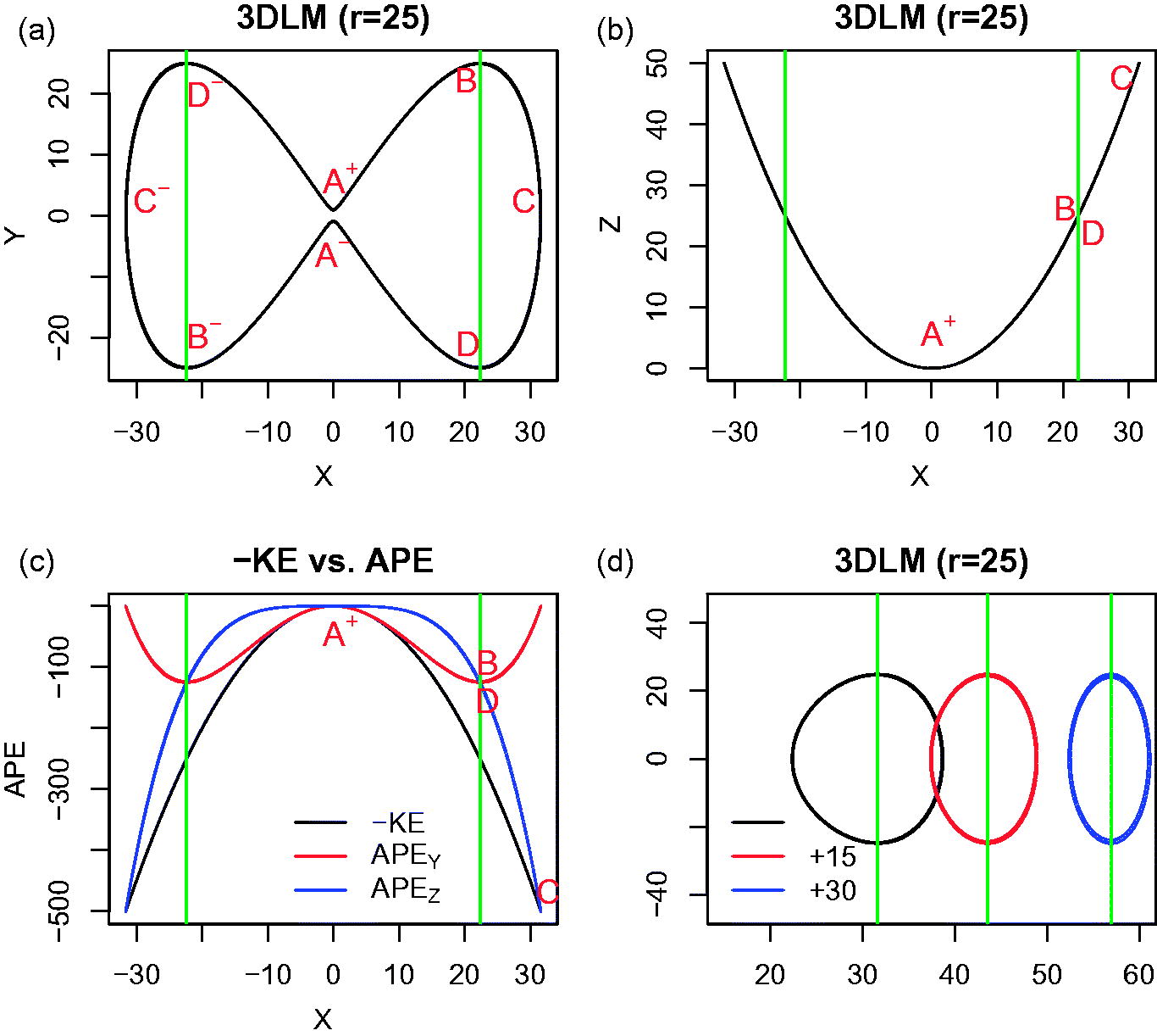
Fig. 8.
Solutions obtained from the 3D-NLM (Equations (3)–(5)). (a) X–Y plot. (b) X–Z plot. (c) X-APE plot. The black, red, and blue lines show normalized −KE, APEY, and APEZ, respectively. Green lines are plotted at where Y2 = Z2. (d) The X–Y plot using different initial conditions, (X, Y, Z) = (X0, 0, 0). The black, red, and blue curves represent results using , and , respectively. The three green lines pass through the corresponding critical points at (Xc, Yc) = .
In Fig. 8a, a solution may move ‘around’ the saddle point and the two stable critical points, and its trajectory defines the large cycle. With a different initial condition, a solution may go around one of the non-trivial stable points (, 0), and its trajectory forms a small cycle. For example, Fig. 8d displays results using three different ICs including X0 = , + 15, and + 30 as shown with black, blue, and red lines, respectively. Note that the numerical solution with the first IC was previously compared with the closed-form solution in Fig. 4. The three vertical green lines indicate the locations of the corresponding stable critical points at Xc = . Solutions in Figs. 8a and 8d suggest that the larger the value of (initial) Xo is, the further the trajectory may move away from the saddle point. When an initial Xo is distant from zero (i.e. the saddle point), nonlinearity may become dominant as compared to the (linear) heating term. The corresponding solutions (e.g. the blue curve in Fig. 8d) become more symmetric with respect to the green line that passes through the nontrivial stable critical point.
Figure 9 provides the time evolution of and for the solutions in Figs. 8a–8c. The energy cycle: (1) begins near point A, at A+ = (0,0+) to be specific; (2) goes through B, C, and D; and 3) returns back to A, (i.e., A− = (0,0−)). In Leg A–B, where the linear (heating) force dominates, the solution X grows gradually with {, } and . The upper arrow (↑) and the down arrow (↓) are, respectively, used to indicate an increase and decrease. In Leg B–C (or C–D), where the nonlinear restoring force becomes dominant, the solution X increases (or decreases) rapidly with {, } (or {, }) and . In Leg D–A, solution X decays slowly with {, } and . Once the trajectory returns back to point A–, it may experience another small cycle, going to B–, C–, and D– and returning back to point A+. Here, , and . The two ‘small cycles’ form the large cycle, and the time evolution of energy is the same for both wings.
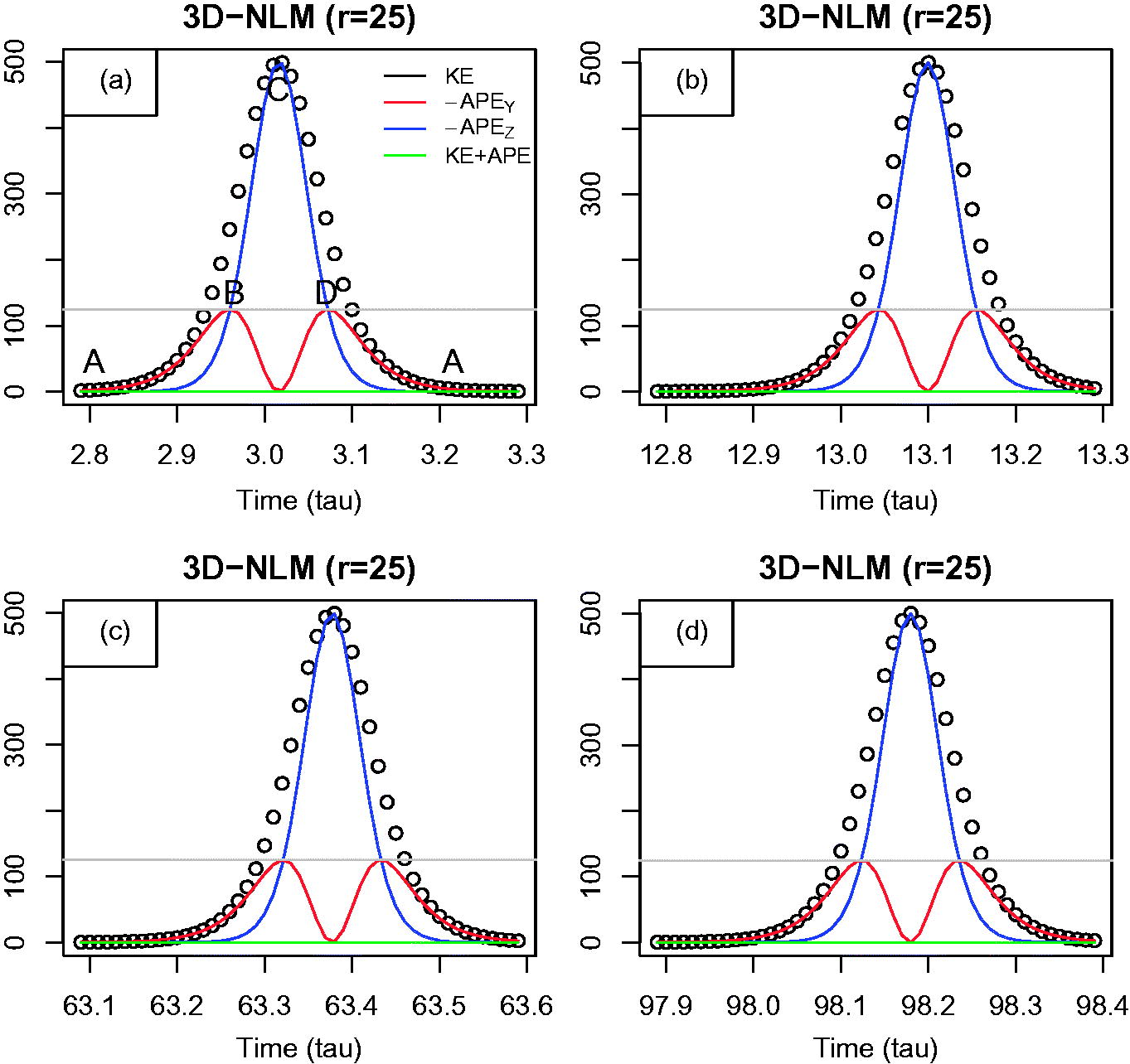
Fig. 9.
Time evolution for the KE and APE in the 3D-NLM (Equations (13)–(14)). Black open circles display KE. Red, blue, and green lines indicate −APEY, −APEZ, and KE + APE, respectively. All of the fields are normalized by Co. The gray line is plotted at a value of σr/2, which is equal to −APEY/Co and −APEZ /Co at X = Xt. These panels show that the solutions are oscillatory and periodic.
Concluding remarks
4.
More than 50 years ago using his forced, dissipative model, Lorenz showed that chaos may appear in the presence of nonlinearity, suggesting that nonlinearity may be the source of chaos. In this study, using the non-dissipative Lorenz model (3D-NLM), we discussed how nonlinearity may act as a restoring force to produce oscillatory solutions. We first presented the closed-form solution of the nonlinear equation , which is derived from the 3D-NLM with r = 0. The corresponding solution is oscillatory (wave-like) and the nonlinear term (X3) is associated with the nonlinear feedback loop. Therefore, we suggest that the nonlinear feedback loop may act as a restoring force. The closed-form solution obtained using a trigonometric function (Equation (18b)) compares well with the closed-form solution obtained using an elliptic function (Equation (C9)); and the simplicity of the former effectively illustrates the fundamental role of nonlinearity in producing oscillatory solutions.
While a heating term is considered, a linear analysis shows a saddle point at the origin and two stable non-trivial points (i.e. two centers) at . Here depends on the product of σ and r, as well as the initial conditions. In addition, three types of solutions could be obtained. Two of the solutions display periodic movement around one non-trivial critical point or all three critical points. The corresponding trajectories are orbitally stable. The third type of solution is the so-called homoclinic orbit. Two of the trajectories, beginning at points near the homoclinic orbit, may be diverged, displaying the dependence of the solutions on the initial conditions. The homoclinic orbit is not orbitally stable. Note that this solution dependence is different from that associated with a chaotic attractor in a dissipative system that includes two unstable non-trivial critical points.
The homoclinic orbit connects the stable and unstable manifolds of the saddle point, but it is not a periodic solution. However, the time evolution of energy along the homoclinic orbit can qualitatively depict the energy evolution for trajectories that that begin with initial points close to the saddle point and move around a non-trivial critical point. From the perspective of an energy partition, inclusion of the Z mode within the 3D-NLM not only introduces additional APE to be transferred to KE, but it also limits KE to be finite, as compared to the linear system. We illustrated that the relative impact of the nonlinear restoring force and the linear (heating) force determines the partition of the averaged available potential energy associated with the Y and Z modes, denoted as and , respectively. Based on the energy analysis, an energy cycle with four different regimes could be identified with the following four points: , , and . With the initial perturbation, , and . As shown in Fig. 6, the energy cycle may: (1) begin at (near) point A; (2) go through B, C, and D; and (3) return back to A. appears when solutions are strongly nonlinear (i.e. in Legs B–C and C–D), suggesting that inclusion of the Z mode can enable the partition of APE on different scales, leading to nonlinear solutions. Since point A is a saddle point, the ‘cycle’ is only half of a large cycle, representing one wing of the glass-winged butterfly. More detailed discussions of the energy cycle and the large cycle are provided near the end of Section 3.
In summary, the nonlinear feedback loop alone may act as a restoring force and the heating term alone can produce a saddle point within the 3D-NLM. The nonlinear feedback loop and the heating term collectively lead to three critical points and three types of solutions. The existence of oscillatory solutions reveals the role of the nonlinearity (i.e. the nonlinear feedback loop) in producing recurrence and the appearance of the homoclinic orbit suggests the divergence of two nearby trajectories. This type of solution dependence on ICs will be examined and compared with the one associated with a chaotic attractor in the 3DLM and high-dimensional LMs in a future study.

Fig. C1.
A comparison of the nonlinear oscillatory solutions using r = 0 in Equations (18b) and (C9), expressed using an elementary trigonometric function and an elliptic function, respectively. (a) The solution of Equation (18b) in red. (b) The solution of Equation (C9) in blue. (c) Both of the solutions in (a) and (b). (d) Differences of the two solutions.
Acknowledgments
We thank Prof. Zdzislaw Musielak, Dr. Kayo Ide, Dr. Tzi-Cheng Lai, Prof. Xubin Zeng, Prof. Ricardo Carretero, and Prof. Juan Serna for valuable comments and/or discussions, and Jill Dunbar for proofreading the manuscript.
Disclosure statement
No potential conflict of interest was reported by the author.
Appendices
Appendix A
Derivations of Equation (3)
In this section, we describe the procedures used to derive Equation (3). As discussed in Shen (2014), the nonlinear advection term in Equation (1) does not explicitly appear within the Lorenz model. Therefore, Equation (1) can be written as follows:
Using the of Shen (2014), ψ and θ can be represented as:
Here, C1 and C2 are defined in Equation (9) of Shen (2014). Note that the two constants C1 and C2 are different from those in Equations (13) and (14). Next, the left- and right-hand side terms of Equation (A1) are expressed using , respectively, as follows:
Here, l and m, as defined in Shen (2014), represent the horizontal and vertical wavenumbers, respectively. Substituting Equations (A4) and (A5) into Equation (A1), we have:
We define a time scale (To) as:
and obtain:The term H represents the domain height, and a is the ratio of the vertical scale of the convection cell to its horizontal scale, (i.e. ). With Equation (9) in Shen (2014), the right-hand side of Equation (A6) becomes:
With Equation (A9), Equation (A6) becomes:
The above equation then becomes Equation (3), when is assumed.
Appendix B
Nonlinear feedback loop and nonlinear restoring force
The non-dissipative Lorenz model (3D-NLM) with no heating term is written as:
Note that the above equations represent a special system with a very large r for the original 3DLM (e.g. Sparrow, 1982; Strogatz, 2015). Equations (B1)–(B2) lead to
From Equation (B1) and (B3) (i.e. X * Equation (B1)− σ*Equation (B3)), we have
and where C is a constant. The initial condition of leads to C = 0. Therefore, Equations (B4) and (B5) with the above initial condition gives usThe above derivations illustrate the relationship between the X3 and the nonlinear feedback loop (i.e. –XZ and XY), which are associated with a pair of up-scaling and down-scaling processes as discussed in Shen (2014). Note that replacing and (XY) by (XZ) and in Equations (B2) and (B3), respectively, we obtain the real-valued Maxwell-Bloch equations (Equations (1.20)) of David and Holm, 1992). Therefore, it is suggested that the pair of (XZ) and serves as a restoring force in the Maxwell–Bloch equations.
Appendix C
A closed-form solution for r = 0 using elliptic functions
Nonlinear dynamics have been widely studied using solutions to the nonlinear Duffing equation. The Duffing equation that governs certain damped and driven (i.e. dissipative and forced) oscillatory motions (Bender and Orszag, 1978; Jordan and Smith, 2007; Wikipedia) is given by:
where δ, α, β, γ, and ω are constants. When and and , Equation (C1) appears in the form of the 3D-NLM (Equation (15)). While an exact solution to the general form of the Duffing equation may not have been determined, closed-form, approximated, or numerical solutions have been documented in the literature. In this section, we discuss how closed-form solutions to the special case of the non-dissipative and unforced Duffing equation (i.e. and ) can be obtained and expressed in terms of elliptic functions (Davis, 1960).The incomplete elliptic integral of the first kind, , is written as:
The elliptic functions of the Jacobi are defined as the inverse of the elliptic integral, as follows:
The elliptic functions have the following properties:
and their derivatives can be obtained as follows: andEquations (C4) and (C5) can be helpful for obtaining a solution to the equation (Equation (18a)). Using Equation (C5) and , the solution can be written as:
Through Equation (C6) and , the solution becomes:
Here, D1, D2, θ1, or θ2 are constants and are determined from the initial conditions. θ1 or θ2 can be expressed in terms of complete elliptic integrals of the first kind, , which is calculated using Matlab (http://www.mathworks.com/help/matlab/ref/ellipke.html). In addition, as a result of the definition of the elliptic integral (Equation (C2)) and/or validity of the numerical algorithms for the elliptic functions, k2 may not be equal to –1. Therefore, only Equation (C8) is discussed below. In this study, the IC with and ) = 1 (i.e., )) leads to the following solution with θ2=3K and :
Figure C1 displays solutions obtained from Equation (18b) (Fig. C1-a) and Equation (C9) (Fig. C1-b) and their differences (Fig. C1-d). The solutions are very close. This comparison confirms the validity of the method for obtaining closed-form solutions for the 3D-NLM with r = 0 using elementary trigonometric functions (Fig. 2) that are used to illustrate the role of nonlinearity in producing oscillatory solutions. For the case of α≠0 (i.e. r≠0), similar procedures can be applied using Equation (C5) or (C6) in order to obtain closed-form solutions. The procedures are beyond the scope of the present study.
Appendix D
Equations for the solution of the homoclinic orbit
Here, we present equations that are used for obtaining an analytical solution that begins and ends at the saddle point. Equations (13)–(14) with the ICs (X,Y,Z)=(0,0,0) become:
which lead to:Using the above with Equation (3) yields:
The term X4 in Equation (D4) can be shown to be equivalent to the term X3 in Equation (15) that is associated with the nonlinear feedback loop. Without this term, the system in Equation (D4) or (15) becomes linear. Applying the method described in Chapter 3 of Jordan and Smith (2007), we obtain an analytical solution to the nonlinear system in Equation (D3) that begins and ends at the saddle point (0,0,0), which are shown in Equations (34a)–(34c).