
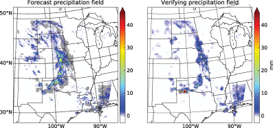
Fig. 1.
An example of a slightly misplaced forecast precipitation field.
Notes: The forecast field (left) is the 24-h forecast of the 1-h accumulated precipitation starting at 0000 UTC 1 June 2005 and the verifying analysis field (right) is the 1-h accumulated Stage II precipitation analysis. In the left panel, the grey shades indicate the contours of the verifying precipitation field.
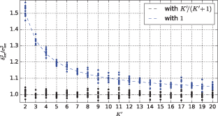
Fig. 2.
Illustration of the effect of the normalization factor K′/(K′ + 1) on the ratio of the estimates of the right- and left-hand sides of Equation (20).
Notes: The values shown are based on randomly generated samples of 10, 000 realizations of , , , assuming a Gaussian random distribution with mean . Because of the sampling fluctuations, the simulation is repeated 10 times for each value of K′ and the results are shown by scatter-plots.
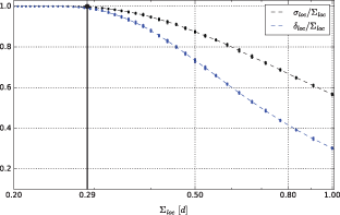
Fig. 3.
The dependence of the prediction σloc and the estimate δloc on Σloc for a finite size search region.
Notes: The values shown are based on a randomly generated sample of 1000 realizations of , , , assuming a truncated Gaussian random distribution with mean in a one-dimensional search domain of size 2d. The values of Σloc on the x-axis are shown using the search radius d as unit, while the values of σloc and δloc on the y-axis are normalized by Σloc.
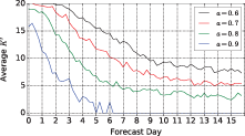
Fig. 4.
Evolution of the average of K′ over all forecast cases for different values of a in the range from 0.6 to 0.9.
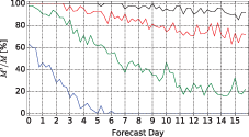
Fig. 5.
Evolution of the percentage M′/M of the forecast cases for which K′ ≥ 2 for different values of a in the range from 0.6 to 0.9.
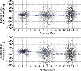
Fig. 6.
Top: the values of for the individual ensemble forecasts (dark blue dots) and the evolution of the estimate of the meridional component of the location bias with the forecast lead time, bottom: the values of for the individual ensemble forecasts (dark blue dots) and the evolution of the estimate of the zonal component of the location bias .
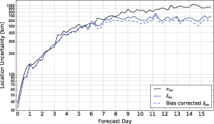
Fig. 7.
The evolution of σloc (solid black), δloc (solid blue) and bias-corrected δloc (dashed blue) with the forecast lead time.
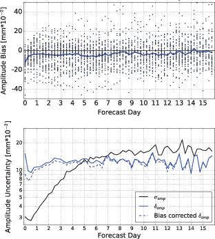
Fig. 8.
Top: the values of for the individual ensemble forecasts (dark blue dots) and the evolution of the estimate of the amplitude bias with the forecast lead time, bottom: the evolution of σamp (solid black), δamp (solid blue) and bias-corrected δamp (dashed blue) with the forecast lead time.