
Introduction
1.
The standard sequential data assimilation (DA) framework assumes that the time is discrete, and that observations assimilated at each time step are made at the analysis time. In practice, the time intervals between consecutive analyses can be substantial, and model states within the observation window can be quite different. It is often important in such cases for a DA method to take into account, in one way or another, the timing of observations. The method is then referred to as asynchronous, in contrast to its standard sequential formulation, which is referred to as synchronous.
The ensemble Kalman filter (EnKF, Evensen, 1994) is based on the Kalman filter (KF), which is a sequential method; however, in the linear perfect model case, the EnKF can be easily adapted to accommodate the asynchronous DA (ADA). Consider the associated minimisation problem:
Here the lower index i refers to time , is the model state, – the initial state estimate, – the initial state error covariance estimate,1 – observations, and – the corresponding observation operator and observation error covariance matrix, is the model resolvent that maps the state from time to ; the norm notation is used.In order to simplify the notations, we define as the block diagonal matrix (or operator) made of the square matrices (or square operators) . We also define as the matrix (or operator) that stacks the matrices (or operators) that are assumed to have the same column number. With these notations, the cost function (1b) can be written as follows:
where
are the concatenated observation vector and corresponding observation error covariance matrix, respectively, and the forward map relates the initial state to the observations:
Apart from the forward map (5) that yields forecast observations at times , the cost function (2) has the same form as that for a single DA cycle with synchronous observations. Consequently, in the linear case, when the tangent linear forward operator (the sensitivity of observations to the initial state) does not depend on , the cost function (2) can be minimised using existing EnKF solutions, provided that the standard (synchronous) observation functions are replaced by the generic forward function (5):
where is the EnKF ensemble; upper “f” refers to forecast; denotes the forecast ensemble observations and is the initial ensemble. In practice, this means that to assimilate asynchronously with the EnKF one simply needs to calculate ensemble observations using forecast ensemble at observation time (Sakov et al., 2010). There are no specific restrictions on in (2) – in particular, it does not have to be block-diagonal – therefore in theory observation errors can be correlated in time within a DA cycle.
Before formulated in Sakov et al. (2010), the recipe (6) has been used in a scheme called 4D-LETKF (Hunt et al., 2007), where it was empirically derived from a method called 4D-EnKF (Hunt et al., 2004).
In practical terms, the ADA makes it possible to avoid storing the full ensemble at each observation time, storing only ensemble observations instead. Because in large-scale geophysical systems the model size is typically much larger than the number of observations, this yields a significant economy of resources.
Formulation () of the minimisation problem implies assimilation time ; however, one interesting feature of the EnKF in the linear perfect model case is the time invariance of the optimising ensemble transform. If the update is conducted at time by applying transform to a forecast ensemble ,
then, to the same effect, it can be applied at other time :
This time invariance of the ensemble transform has been used in the ensemble Kalman smoother (Evensen, 2003) and made it possible to interpret the ensemble transform as a linear combination of the ensemble trajectories in the 4D-EnKF (Hunt et al., 2004).
The above framework for the ADA with the EnKF is based on two important assumptions: linearity and perfect model. While the KF is a linear method, it can be (and indeed is) successfully applied to weakly nonlinear cases, when the Jacobians and do not change much through the DA cycle and over the characteristic uncertainty range of the state. The same principle motivates the applicability of the approach (6) to the ADA with the EnKF. This is why we kept the nonlinear notation for the forward operator.2 In strongly nonlinear cases, the method is, generally, no longer applicable, and iterative minimisation algorithms (e.g. Gu and Oliver, 2007; Bocquet and Sakov, 2014) must be used.
The situation in the case with the model error is somewhat similar. Various aspects of additive deterministic (possibly time-correlated) model error and how formulation () should be generalised have been considered in Lorenc (2003), Trémolet (2006) and Carrassi and Vannitsem (2010). However, because (1c) assumes a lossless transfer of information between DA system states in time by the model, it has not been clear whether the concept of the ADA can still be useful in cases with substantial model error. Recently, an iterative method for strongly nonlinear systems with additive stochastic model error called IEnKF-Q has been proposed (Sakov et al., in press) that successfully employs combining propagated ensemble anomalies and model noise ensemble anomalies into a single ensemble of anomalies to obtain an algebraically simple solution for the Gauss–Newton minimisation. The authors suggested that a similar approach can possibly be used to generalise the concept of the ADA with the EnKF in the case of additive model error. This study proposes such a generalisation.
The minimisation problem
2.
Below we mainly follow the formulation and approach to the solution of the minimisation problem from Sakov et al. (in press), with the aim to put up an analogue of the recipe (6) that would permit a simultaneous assimilation of observations made at different times in the case of additive model error without loss of optimality. Sakov et al. (in press) considered a single DA cycle starting at time with observations at , while we consider a cycle with an arbitrary number of model steps:
Here is the initial state (the analysis from the previous cycle), – the initial state error covariance, – the model error covariance at , and upper star refers to the solution of the minimisation problem.From a statistical perspective, (9b) relates to the joint probability density function on state and observation vectors since coincides with up to a constant. This implies that the model noise, as random variable, is assumed Gaussian, unbiased, of covariance matrix at and uncorrelated in time (see Carrassi and Vannitsem, 2010, for a generalisation).
Let the covariances and be factorised by the corresponding ensemble anomalies and :
where is a vector of entries 1. In many applications, the representation of model errors through the anomalies is more natural and convenient than through the . A discussion on this specific topic can be found in Section 4 of Sakov et al. (in press). Let us seek the solution of the minimisation problem () in the ensemble space of these anomalies: The weights are similar to the control variable in the ‘forcing’ formulation of the weak-constraint 4D-Var (see Equation (2) in Trémolet, 2006), although using instead of has a convenience of diagonalising .The problem () becomes equivalent to
Let us concatenate into :then (12b) becomes
where and are given by (3) and (4), and
The cost function (14) is similar to the formalism developed by Lorenc (2003) or to Equation (11) of Desroziers et al. (2014), but differs in that it is not incremental and can be obtained directly.
In (14), is a function of because of (). Let us expand in power series of and retain the linear term only:
where3
and
Here the ensemble anomalies are completed by zeros so that they all have the same number of columns as . Note that the augmentation of the propagated state error anomalies and model error anomalies has also been used in the reduced rank square root filter by Verlaan and Heemink (1997) in their Equation (28). Substituting (17) into (14) yields a form convenient for Gauss–Newton minimisation:where
In the nonlinear case, (20) can be minimised by Gauss–Newton iterations. This involves using the approximate Hessian obtained by neglecting nonlinear terms . In the linear case, the cost function becomes quadratic, and the solution is given by:
where denotes the unique positive (semi)definite square root of a positive (semi)definite matrix, and is an arbitrary mean preserving orthonormal matrix4: .These equations provide the update of the ensemble at all time levels. Similarly to the perfect model case, the same coefficients and the same ensemble transform are used over the whole assimilation window. However, due to the augmentation of the propagated ensemble anomalies with model error anomalies in (19c), the updated trajectories of the initial ensemble are no longer continuous in time.
Asynchronous DA
3.
Based on the solution of the minimisation problem in the previous section, we can now formulate a framework (rules) for the ADA with the EnKF in presence of additive model error. According to equations (), to update the system state, one needs to calculate the forecast observations and forecast ensemble observation anomalies ; they in turn allow one to calculate the Hessian (approximate Hessian in the nonlinear case), coefficients and transform . Therefore, the essence of the ADA with the EnKF can be formulated as follows:
where is defined by (19b) and (19c).
Subject to the new evolution equation for ensemble anomalies (19c), the rules (21) and (23) can be interpreted in the same way as in the perfect model case: calculate ensemble observations using the forecast ensemble at observation time.
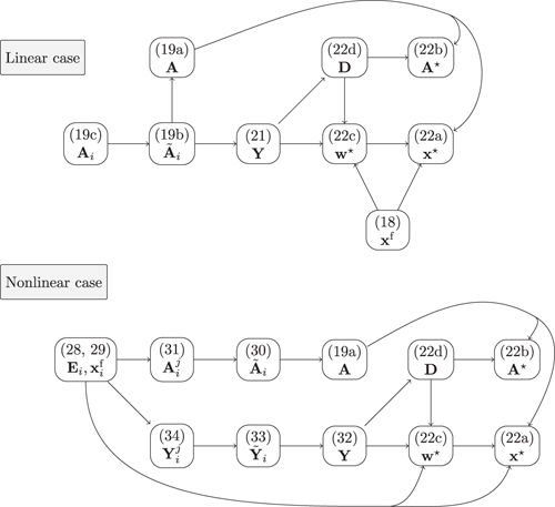
Figure 1.
The sequence of the complete analysis cycle in both the linear (upper) and the nonlinear (lower) case. From left to right, the nodes indicate the equation to use as referred to in the paper and the yielded quantities. The second, lower chain in the nonlinear case is needed if the observation operator is nonlinear. Arrows mean that the computation of the target node content requires the content of the origin node.
The sequence of the complete linear analysis cycle is synthesised in Fig. 1 (upper panel).
Discussion
4.
Increasing ensemble size
4.1.
The update equations () have the same form as in the perfect model case; however, the propagation of the ensemble anomalies in (19c) is substantially different. According to (19c), in presence of model error, the forecast ensemble of anomalies is not only transformed with the tangent linear model, but is also augmented with the corresponding ensemble of model error anomalies. This procedure implicitly implements the forecast covariance equation of the KF
so that , and manifests an effective increase of the ensemble size at every time step:
where is the size of ; is the size of and is the size of , i.e. the initial ensemble size. The practical choice for the has been discussed in Section 4 of Sakov et al. (in press).
Note that this increase of the ensemble size may not be strictly necessary for implementing (24). For example, if the column space of is a subspace of the column space of , then adding model error covariance can be done without changing the ensemble size. Yet, the augmentation of the state error and model error ensemble anomalies in (19c) is an essential part of the described minimisation procedure, regardless of whether it is possible to factorise the forecast state error covariance with a smaller ensemble or not. It enables to concatenate the vectors of ensemble weights into a single vector in (13) so that each component of this vector acts only on the columns of the augmented ensemble associated with the model error added at time (except that is indeed associated with the initial state error). In this way, the minimisation uses the same vector of coefficients over the whole observation window, similarly to the perfect model case.
Nonlinearity and approximation of and
4.2.
Although the EnKF is a linear method targeting weakly nonlinear systems, it is still desirable to optimise it for strongly nonlinear situations, for two reasons. Firstly, it is quite common for a weakly nonlinear system to become strongly nonlinear during relatively short and infrequent transition periods. Secondly, there are a variety of EnKF-based iterative methods for strongly nonlinear systems that would benefit from such an optimisation.
The EnKF is a derivative-less method: it approximates the Jacobians and based on application of the forward function to the ensemble of model states . In the linear case, the results of these approximations do not depend on the ensemble spread; in the nonlinear case to achieve correct sampling of nonlinear effects, the magnitude of the ensemble anomalies should be of order of the standard deviation of the state error. For a system with additive model error, this means that the forecast error anomalies should have magnitude similar to that of samples from , where the forecast covariance is given by (24).
Such sampling can be associated with the statistical estimator of the covariance,
where is an ensemble of anomalies. Using this factorisation yields the characteristic magnitude of the anomalies of the order of its standard deviation, regardless of the ensemble size.
The minimisation procedure in Section 2 uses a different factorisation,
which simplifies the algebraic side. Using this factorisation reduces the characteristic magnitude of anomalies with increasing ensemble size. To obtain anomalies of physically ‘right’ magnitude, one needs to scale them up with a factor of , but only if all samples in the ensemble are drawn from the same pool. If, for example, we introduce a new ensemble
then we should still scale it with rather than with , where is the size of .
Because the magnitudes of the anomalies and in (19c) cannot be assumed to be similar, it seems technically challenging to put up a generic re-scaling procedure for switching between factorisations (26) and (27) in the course of minimisation. This leaves us the following two main options.
(1) Using factorisation (27) over the whole DA cycle, which means no rescaling before or after application of nonlinear functions and . This approach underestimates the ensemble spread in approximations and shifts the minimisation towards the Newton method from the more inherent for the EnKF (and generally more robust) secant method.
(2) Scaling components of appended at different time steps according to the size of these components before application of and , and scaling back after that. This approach still does not make all anomalies of being sampled from , but can be a good practical compromise. It is elaborated below.
where is the initial ensemble and
We then define the new anomalies that yield via (). They are composed of sub-blocks , each of them corresponding to the ensemble appended at time :
where
The submatrix corresponds to the first columns of ; , for , corresponds to the submatrix from column to column of .
The forecast observation anomalies (21) are then calculated as
where
and
To summarise, the sequence of the complete nonlinear analysis cycle is synthesised in Fig. 1 (lower panel).
Observations correlated in time
4.3.
The formulation of the minimisation problem () assumes that observations at different times are noncorrelated, so that the merged observation error covariance matrix in (4) is block-diagonal; however, we can see no problem in removing this restriction, that is assuming that the observations within a DA cycle can be time correlated.
Ensemble resizing
4.4.
One practical implication of the proposed framework for ADA in presence of additive model error is the need for ensemble resizing at the end of a cycle to cut back the increased ensemble size due to (19c). If the augmented ensemble has the same rank as , then the ensemble size reduction from to can be performed losslessly (that is, without changing the analysed state error covariance). In large-scale geophysical EnKF systems, the ensemble size is always much smaller than the model size, and realistic implementations of model noise can be expected, generally, to project onto the left null-space of the ensemble. In this case, the resizing will involve removing the principal components with the smallest variance (Verlaan and Heemink, 1997; Raanes et al., 2015; Sakov et al., in press).
Observation time binning
4.5.
The minimisation problem () associates each time step with observations and model error . In practice the observations can be distributed in time continuously. They will need then to be binned by some time intervals, and model error estimates will need to be prescribed for each of these intervals. Because of the overhead associated with augmenting the ensembles of model error anomalies into the ensemble anomalies by (19c) one may have to use a rather coarse time binning for the model error. It is then possible to assume that the forward function in (34) propagates ensemble to the time of each particular observation, as the overhead associated with the time binning of ensemble observations can be much smaller. This is the same observation time binning strategy as the one proposed by Trémolet (2006) with his Equation (9).
ADA: further extending the KF
4.6.
The EnKF yields a large number of advantages over the KF: scalability, derivative-less formulation, ease of implementing the covariance propagation equation, robustness, and so on. Most of these advantages can be viewed as concerning the technical side of the Kalman filtering. By contrast, the ADA aims at extending the very framework of the sequential DA. While in the perfect model case it is possible to modify the square root formulations of the KF to permit the ADA similarly to that in the EnKF, the technique proposed in this note involves using nonsquare covariance factorisations of varying size within a DA cycle. We see it as yet another step in the evolution of the KF-based methods towards greater universality, well beyond the original scope of the KF.
Summary
5.
Equations (23), (21) and (19c) provide a framework for the ADA with the EnKF in presence of additive model error. Its derivation in the course of solving the minimisation problem warrants its optimality in the linear case.
The most essential new component of the proposed framework is Equation (19c) for propagation of ensemble anomalies. This equation manifests an effective increase of the ensemble size at each time step by the size of the ensemble of model error anomalies. We argue that this increase is necessary for the optimal ADA in presence of additive model error regardless of whether the model error anomalies project onto the column space of the ensemble or not; in practice, it deems it necessary to resize the ensemble at the end of the cycle.
Disclosure statement
Notes
[2] The upper label ‘a’ refers to analysis as, later on, these initial state and error covariance matrix will coincide with the outcome of a previous analysis.