
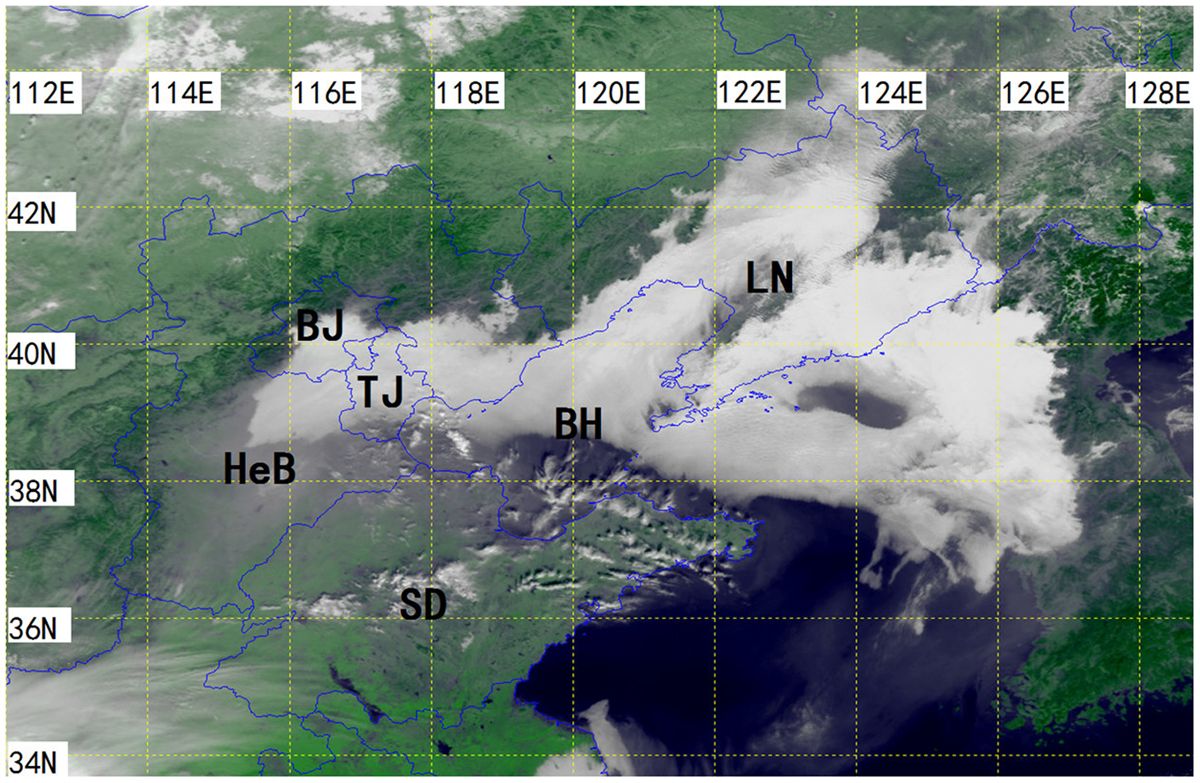
Fig. 1.
Satellite visible image from NOAA-17 at 02:28 UTC 21 February 2007. The grey filled region with a sharp boundary indicates the fog coverage. Abbreviations used: LN = Liaoning Province, BJ = Beijing, TJ = Tianjin, BH = Bohai Sea, HeB = Hebei Province and SD = Shandong Province (refer to Fig. 1 of Hu et al. (2014)).
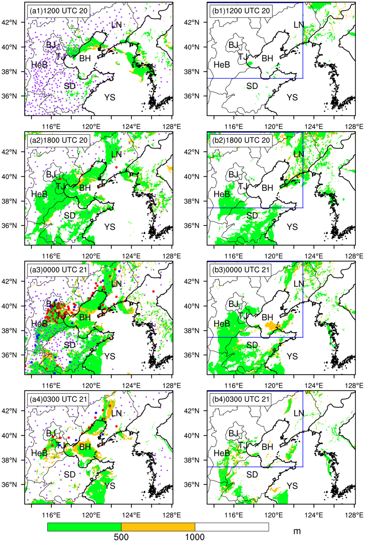
Fig. 2.
Fog coverage (vis < 1000 m) from the simulation of the Truth Run (left) and BG Run (right, shading) at 12:00 UTC (a1, b1), 18:00 UTC (a2, b2) 20 February and 00:00 UTC (a3, b3) and 03:00 UTC 21 (a4, b4) February 2007, respectively, at the first model vertical level in the innermost model domain, and from the visibility observations by the surface stations (dots). The red, blue and purple dots denote observed visibility for the range of <500 m, 500–1000 m and > 1000 m, respectively. Abbreviations are the same as Fig.1.
Table 1.
The comparison of different observation types for both D02 and D03.
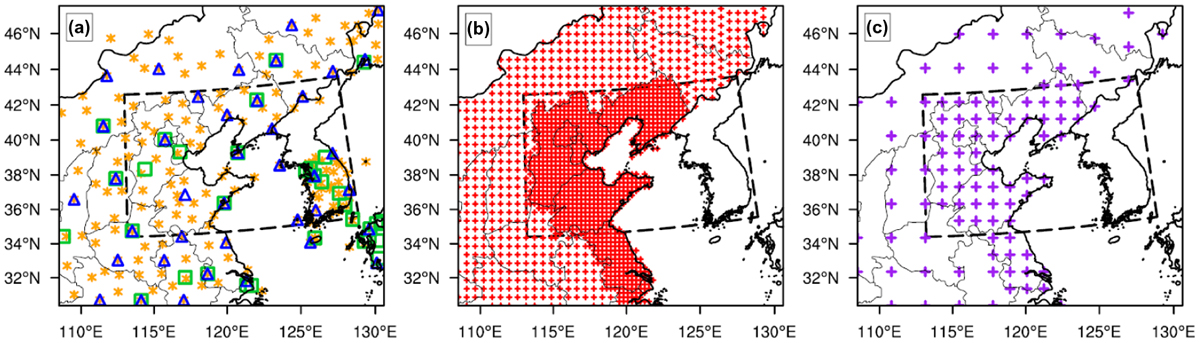
Fig. 3.
The real locations of rawinsonde (blue triangle), SYNOP (orange asterisk) and METAR (green square) (a), the hypothetical locations of AWS (red cross) (b), and PBL wind profilers (purple cross) (c) in China inland regions within D02. The box with black dashed line is the area of D03.
Table 2.
Observation errors of rawinsonde and wind profiler.
Table 3.
List of experiments.
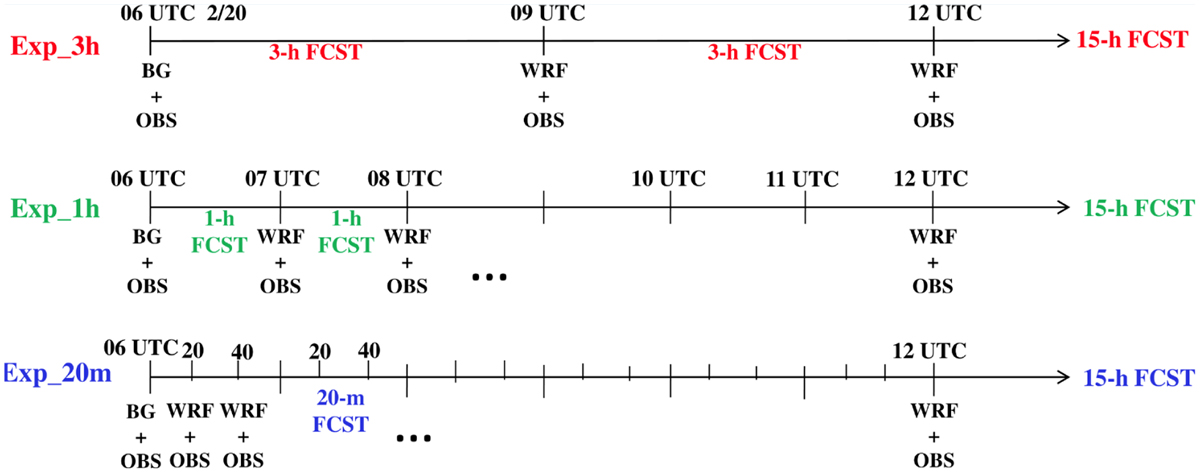
Fig. 4.
Schematic diagram of Exp_3h, Exp_1h and Exp_20m. BG means first guess from the BG Run. WRF means first guess from the model forecast. OBS means observations assimilated.
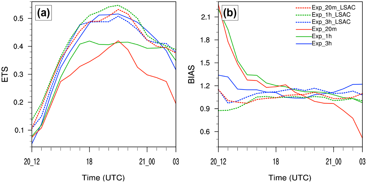
Fig. 5.
Evolutions of area-averaged ETS (a) and BIAS (b) for the experiments using the traditional 3D-Var (solid line): Exp_3h (blue), Exp_1h (green) and Exp_20m (red), and using the modified scheme (dashed line): Exp_3h_LSAC (blue), Exp_1h_LSAC (green) and Exp_20m_LSAC (red) in DNC.
Table 4.
The temporal-averaged ETS of the experiments from 12:00 UTC 20 February to 03:00 UTC 21 February 2007.
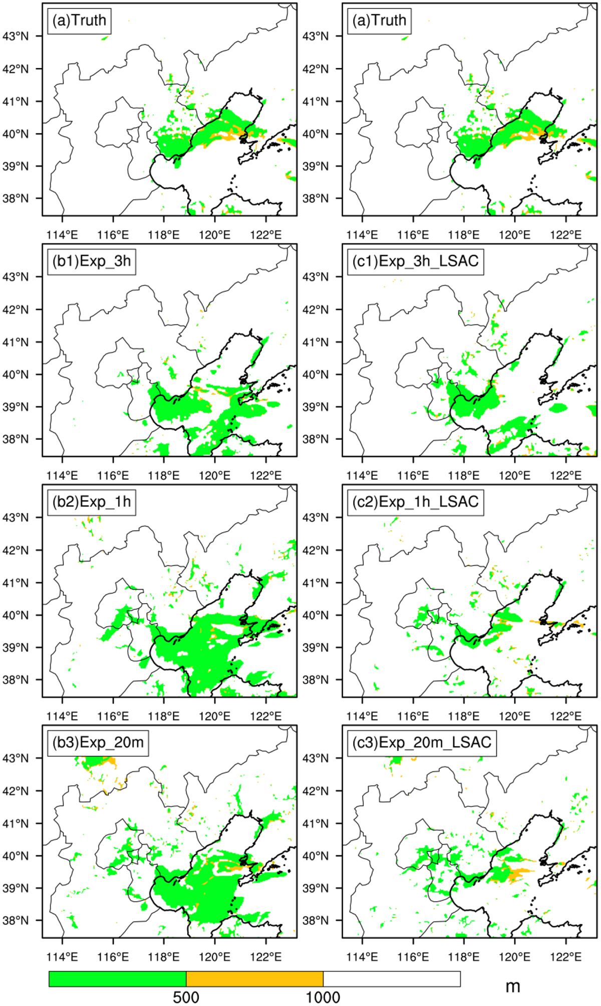
Fig. 6.
As in the blue box of Fig. 2, but for the Truth Run (a) and the experiments Exp_3h (b1), Exp_1h (b2), Exp_20m (b3), Exp_3h_LSAC (c1), Exp_1h_LSAC (c2) and Exp_20m_LSAC (c3) in DNC at 12:00 UTC 20 February 2007 (1 h forecast).
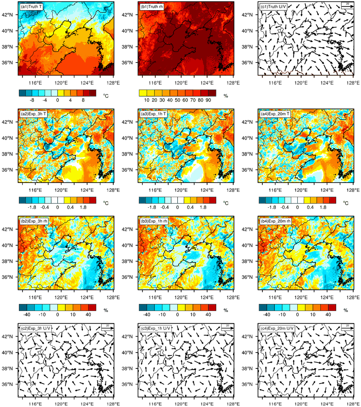
Fig. 7.
The top row: map view of 2-m temperature (a1), the relative humidity (b1) and horizontal wind (c1) at the first model vertical level for the Truth Run; second and third rows: the differences (analysis minus Truth) of temperature (a2–a4) and relative humidity (b2–b4) for experiments Exp_3h (a2, b2), Exp_1h (a3, b3) and Exp_20m (a4, b4); The bottom row: horizontal wind in the analysis for experiments Exp_3h (c2), Exp_1h (c3) and Exp_20m (c4) at the first vertical model level over the finest domain at 12:00 UTC 20 February 2007 (the last DA time).
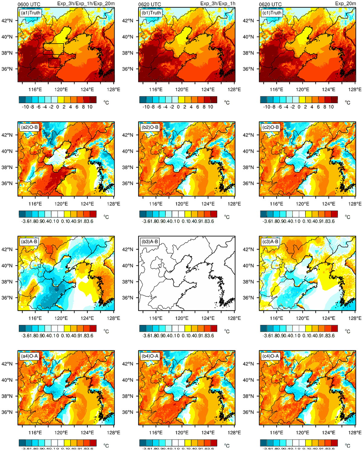
Fig. 8.
Map view of 2-m temperature for the Truth Run (the top row, a1, b1, c1), the differences (background minus Truth, the second row, a2, b2, c2), the increments (analysis minus background, the third row, a3, b3, c3) and the differences (analysis minus Truth, the bottom row, a4, b4, c4) for experiments (Exp_3h, Exp_1h and Exp_20m) at 06:00 UTC (the left column, a1–a4), experiments (Exp_3h and Exp_1h) at 06:20 UTC (the middle column, b1–b4) and experiment (Exp_20m) at 06:20 UTC (the right column, c1–c4) over the finest domain. Note that, although there is actually no DA for Exp_3h and Exp_1h at 06:20 UTC, the forecast field is regarded as both the ‘background’ field and the ‘analysis’ field with the increment of zero to compare with the impact of DA for Exp_20m. The same treatment is used for the following Fig. 11.
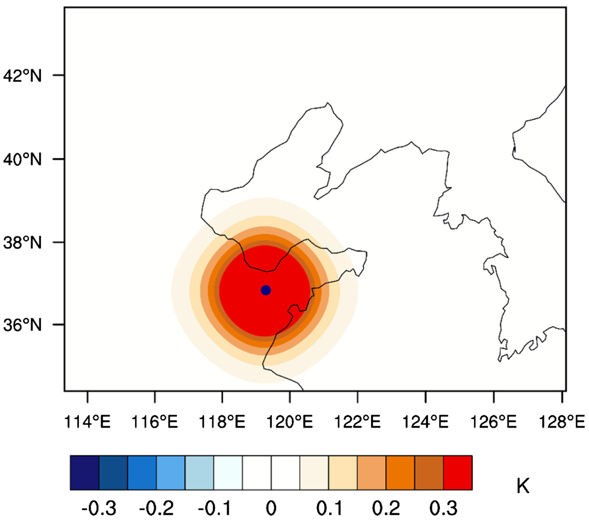
Fig. 9.
The increment of temperature from the single observation test for the temperature field at the first model vertical level at (36.6N, 119.5E) (dark dot) with the innovation of 0.85 K and the background field from the BG Run at 06:00 UTC 20 February 2007.
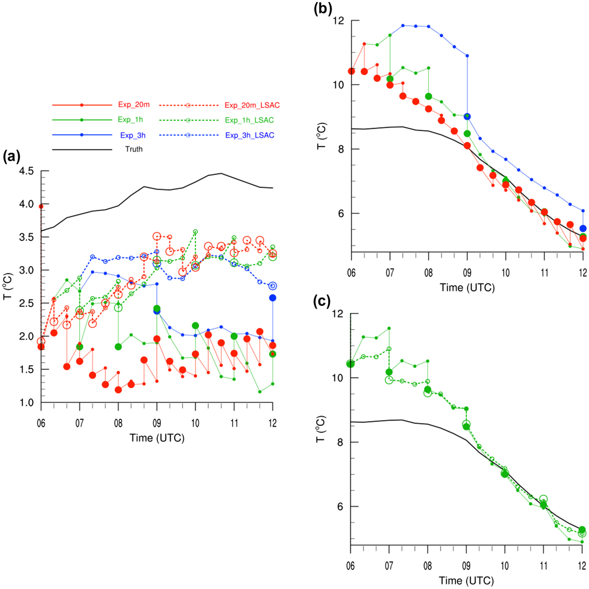
Fig. 10.
(a) evolutions of area-averaged 2-m temperature for the Truth Run (black) and experiments Exp_3h (blue solid), Exp_1h (green solid), Exp_20m (red solid), Exp_3h_LSAC (blue dashed), Exp_1h_LSAC (green dashed) and Exp_20m_LSAC (red dashed) in the background (markerlines) and analysis (large markers) over the top black box shown in Fig. 8a1 from 06:00 UTC to 12:00 UTC 20 February 2007; (b) As in (a), but for the Truth Run and experiments Exp_3h, Exp_1h and Exp_20m over the bottom black box shown in Fig. 8a1; (c) As in (a), but for the Truth Run and experiments Exp_1h and Exp_1h_LSAC over the bottom black box shown in Fig. 8a1.
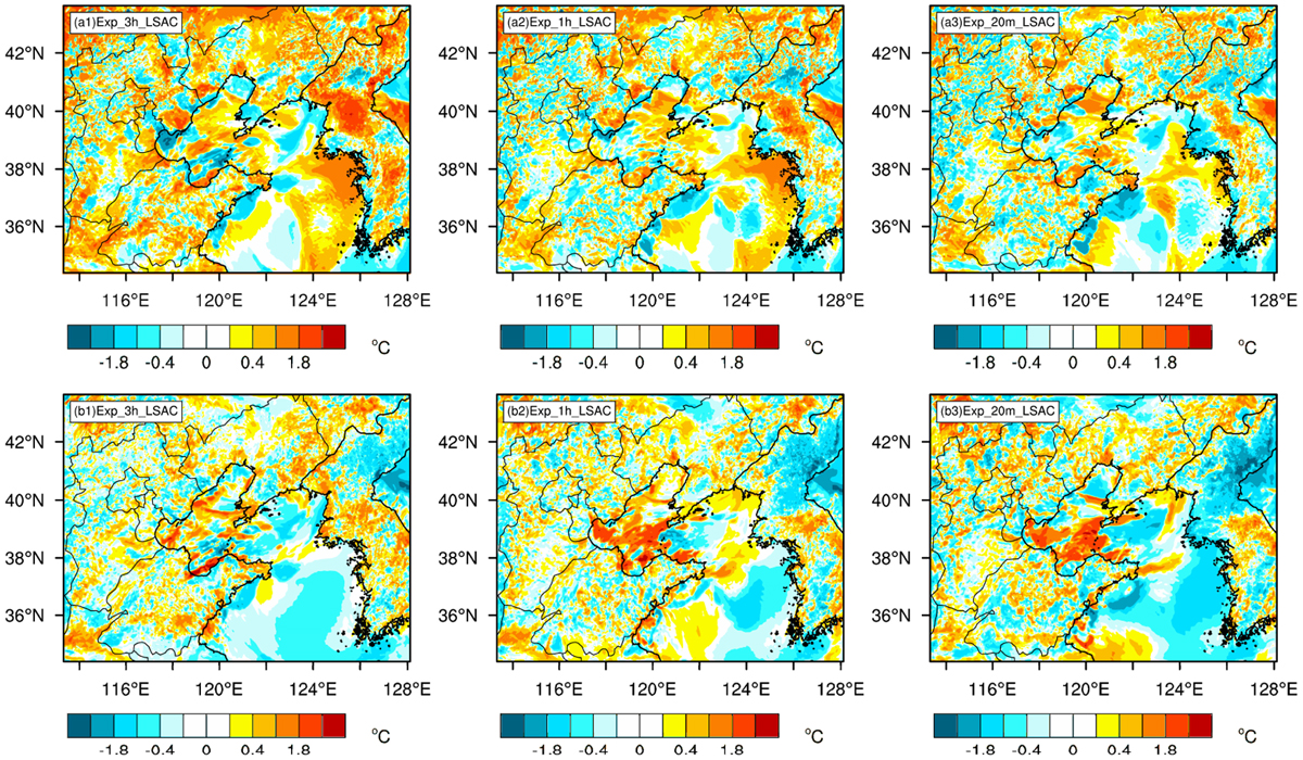
Fig. 11.
The top panel: Same in Fig. 7a2–a4, but for experiments in the modified scheme; The bottom panel: same in Fig. 7a2–a4, but for differences of the analysis between experiments with the modified and the traditional 3D-Var schemes.
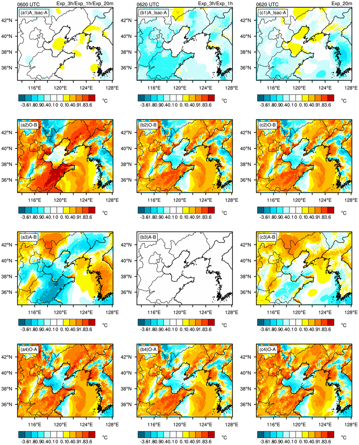
Fig. 12.
The top panel: same in Fig. 8c2–c4, but for differences of the analysis between experiments with the modified and the traditional 3D-Var schemes; The bottom three panels: Same in Figs. 8 for the bottom three panel, but for experiments in the modified scheme.
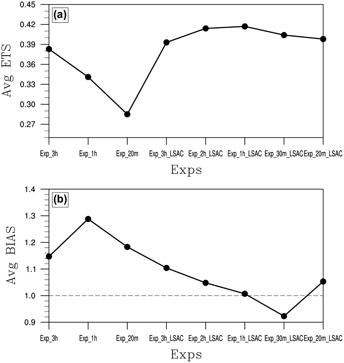
Fig. 13.
The temporal-averaged ETS (a) and BIAS (b) in Fig. 5 for experiments with the traditional 3D-Var scheme (Exp_3h, Exp_1h and Exp_20m) and modified scheme (Exp_3h_LSAC, Exp_2h_LSAC, Exp_1h_LSAC, Exp_30m_LSAC and Exp_20m_LSAC).