The smoother extension of the nonlinear ensemble transform filter

The nonlinear ensemble transform filter (NETF)

2.1.

The purpose of this work is to extend the nonlinear ensemble transform filter (NETF) by a smoother such that the state estimates resulting from the data assimilation take also future observations into account. First, the NETF is reviewed here following Tödter and Ahrens (2015). In the following, the state vector ${\mathbf{x}}_k$ represents the prognostic model variables of a dynamical system $\mathcal{M}$ at time $t_k$. An ensemble consists of m model states, which are stored in the columns of the matrix ${\mathbf{X}}_k=[{\mathbf{x}}_k^{(1)},\dots ,{\mathbf{x}}_k^{(m)}]$, where the superscript (i) denotes the ensemble index. The ensemble filters considered here alternate forecast and analysis steps. The forecast corresponds to an ensemble integration with $\mathcal{M}$. The analysis step transforms the forecast ensemble ${\mathbf{X}}_k^f$ into an analysis ensemble ${\mathbf{X}}_k^a$ that accounts for the current observations. The observations at time $t_k$ are denoted by the vector ${\mathbf{y}}_k$ of size p and the observation operator ${\mathcal{H}}_k({\mathbf{x}}_k)$ maps any model state ${\mathbf{x}}_k$ into observation space.

The ensemble mean at time $t_k$ is computed as ${\overline{\mathbf{x}}}_k=\frac{1}{m}{\mathbf{X}}_k\mathbf{1}$, using the vector $\mathbf{1}={(1,\dots ,1)}^T$ of length m. Thus, defining the matrix

the ensemble perturbation matrix ${\mathbf{X}}_k^{\prime }$ is given by

with

where ${\mathbf{I}}_m$ denotes the $m\times m$ identity matrix.

The NETF transforms the forecast ensemble into an analysis ensemble by applying a weight vector and a transform matrix to the forecast mean and the ensemble perturbations, respectively. As most particle filters, the NETF uses the likelihood weights that derive from Bayes’ theorem, instead of a transformation purely based on covariance matrices as in EnKFs. For normally distributed observation errors with covariance matrix ${\mathbf{R}}_k$, the weight of each ensemble member is given by

where ${\mathbf{y}}_k^{f(i)}={\mathcal{H}}_k({\mathbf{x}}_k^{f(i)})$. As usual in particle filters, the weights are normalised so that they sum up to one. To increase the filter stability, the ensemble perturbations should be inflated by an inflation factor $\mathit{\gamma }>1$ before the weights are computed. As in EnKFs, $\mathit{\gamma }$ needs to be tuned for optimal assimilation results.

The weight vector and transform matrix of the NETF are computed from these weights by

Here, $\mathbf{D}iag({\mathbf{w}}_k)$ is a diagonal matrix that contains the weights $w^{(i)}$ on the diagonal. The analysis ensemble is given by

where the analysis perturbations are computed as

where $\mathbf{\Lambda }$ is an orthogonal matrix. Here, we use a random matrix [see][]Pham2001,Hoteit02a. As an alternative, de Wiljes et al. (2016) recently proposed a deterministic choice for $\mathbf{\Lambda }$, which is not explored here. In addition, the mean is updated via

For the smoother formulation introduced below, Equation (8) is rewritten as a product of the forecast ensemble and a matrix ${\mathbf{G}}_k$. Following Nerger et al. (2014), where the ESTKF was extended to a smoother, the combination of Equations (8)–(10) gives

with

Computationally, the algorithm is very similar to the ensemble transform Kalman filter (ETKF, Bishop et al., 2001) and the ESTKF (Nerger et al., 2012). The nonlinearity of the NETF results from the use of the particle weights (Equation 4) to update the ensemble mean and to transform the ensemble perturbations. Thus, the correction is a nonlinear function of $\mathbf{y}-{\mathbf{y}}_k^{f(i)}$. The weights in the NETF are computed directly from Bayes’ theorem, and are not derived via assumptions of Gaussianity as in the Kalman filter and its variants. With its explicit ensemble transformation, the NETF can be classified as a second-order accurate particle transform filter (de Wiljes et al., 2016). Accordingly, the NETF is expected to provide better state estimates for sufficiently large ensembles than EnKFs in cases where model nonlinearity results in non-Gaussian state error distributions.

More details on the derivation and implementation of the NETF can be found in Tödter and Ahrens (2015) and Tödter et al. (2016).

The nonlinear ensemble transform smoother (NETS)

2.2.

As the NETF itself, the NETS is formulated as a sequential method. Here, it is shown how the NETS results from the general formulation of a sequential particle smoother.

The aim of smoothing is to compute an estimate of the trajectory of states ${\mathbf{x}}_{0:k}$ by assimilating all observations inside the interval $[t_0,t_k]$, where the notation ${\mathbf{x}}_{0:k}$ denotes all states ${\mathbf{x}}_j$ with $j\in \{0,k\}$. In probabilistic terms, one computes an estimate of the probability density function (pdf) $p({\mathbf{x}}_{0:k}|{\mathbf{y}}_{1:k})$ of the state trajectory ${\mathbf{x}}_{0:k}$ given all observations ${\mathbf{y}}_{1:k}$ up to the current time $t_k$. In contrast to filters, the observations at some time $t_k$ are also used to estimate the state at times $t_j<t_k$. Without loss of generality, it is assumed, that the first observation is available at time $t_1$. It is further assumed that the process is a first-order Markov process and that the observations ${\mathbf{y}}_j$ at some time $t_j$ only depend on the specific state ${\mathbf{x}}_j$ at the time. Using Bayes’ theorem on $p({\mathbf{x}}_{0:k}|{\mathbf{y}}_{1:k})$, the equations for a sequential smoother can be derived (see, e.g. Evensen and van Leeuwen, 2000) as

General particle smoothers, which represent the pdfs by an ensemble of particles have been discussed, e.g. by van Leeuwen and Evensen (1996), Kitagawa (1996), and Godsill et al. (2004) . Writing $p({\mathbf{x}}_{0:k-1}|{\mathbf{y}}_{1:k-1})p({\mathbf{x}}_k|{\mathbf{x}}_{k-1})=p({\mathbf{x}}_{0:k}|{\mathbf{y}}_{1:k-1})$, Equation (15) can be formulated as

where the rightmost term will provide the particle weights.

In the particle representation it is

Here, the notation for the particles follows Cosme et al. (2010). The time index is replaced by a double subscript $k_i|k_j$, where $k_i$ denotes the time represented by the state vector and $k_j$ is the latest time from which observations are considered. An augmented particle holding the state information from different times is denoted by an interval in $k_i$ like ‘0 : k’. Thus, ${\mathbf{x}}_{0:k|k-1}^{(i)}$ denotes the $i-$th ensemble member extended with the forecast of the state at the last time step $[{\mathbf{x}}_{0:k-1|k-1}^{(i)},\mathcal{M}({\mathbf{x}}_{k-1|k-1}^{(i)})]$, where $\mathcal{M}$ is the numerical model. The equal weight $m^{-1}$ for each member results here from the resampling in particle filters or the ensemble transformation performed in the NETF. Applying Equation (15) results in modified weights of the particles, thus

with analysis weights $w_k^{(i)}$ given by

Here, only the likelihood $p({\mathbf{y}}_k|{\mathbf{x}}_k)$ needs to be computed as in the NETF while the denominator only serves to normalise the weights so that their sum is one. In a similar way, a fixed-lag particle smoother can be derived, in which the observations are only used to smooth the previous L time steps (see, e.g. van Leeuwen and Evensen, 1996; Khare et al., 2008).

In extended notation by Cosme et al. (2010), the forecast and analysis ensembles at time k are denoted as ${\mathbf{X}}_k^f\equiv {\mathbf{X}}_{k|k-1}$ and ${\mathbf{X}}_k^a\equiv {\mathbf{X}}_{k|k}$, respectively. Likewise, the state at time $t_j$ having assimilated all observation up to time $t_k$ is denoted ${\mathbf{X}}_{j|k}$. For clarity, the superscripts f and a are still used below, even though they are redundant.

For the smoother formulation, it is important to note that the correction of particles at earlier times $t_j<t_k$ is computed using the same weights $w_k^{(i)}$ as for the filter correction at time t. For the NETS this means that the update matrix ${\mathbf{G}}_k$ in Equation (12) is applied to the ensembles at earlier times to perform the smoothing. Thus, the filter is extended to the smoother by updating the whole trajectory instead of only the ensemble at the current time step with the observations at this latest time step.

In the extended notation, the NETF update Equation (11) is

with ${\mathbf{G}}_k$ given by Equation (12).

The smoother is now applied iteratively by using at each filter analysis step, the matrix ${\mathbf{G}}_k$ to smooth the previous ensembles. The solution at some time $k-l$, which includes all observations up to time k, is hence given by the multiplication

At time $k-l$, the smoothed ensemble ${\mathbf{X}}_{k-l|k}^a$ contains the information from all observations up to l time steps in the future. Here, l denotes the so-called smoothing lag, which defines how far into the past observations influence the smoother estimate.

For a linear model, using an infinite lag in a smoother extension of a Kalman filter, i.e. using all observations within the assimilation window and not using localisation, should yield the minimal error (see e.g. Cohn et al., 1994). However, for higher dimensional and nonlinear systems, two factors limit the optimal lag of the filter. First, as mentioned by Cosme et al. (2010), due to the nonlinearity in the model dynamics, a finite lag will usually provide smaller errors in the estimate. This results in an optimal lag as was shown in Nerger et al. (2014). Second, localisation is usually required for the application of the ensemble filters and smoother to high-dimensional systems. However, the elimination of longer range spatial correlations also limits the usable lag (Khare et al., 2008; Nerger et al., 2014).

The commonly used method of covariance inflation also needs to be taken into account in the smoothing. Ensemble filters usually inflate the ensemble spread to account for the lack of model error, to compensate for effects of nonlinearity (see, e.g. Szunyogh, 2014, Sec. 4.2.7.), and because of sampling errors caused by the finite ensemble size. As derived in Cosme et al. (2010), in ensemble smoothers, the covariance inflation should only affect the covariance at the analysis time. Here, this approach is also used for the NETS, to avoid that the inflation factor is re-applied each time the analysis is smoothed, which would lead to an overinflated ensemble.

In ensemble Kalman smoothers, it is common to multiply the matrix ${\mathbf{G}}_k$ by the inverse inflation factor (see Nerger et al., 2014, for details) to remove the inflation. Unfortunately, this simple approach cannot be used in the NETS since its transform matrix depends nonlinearly on the forecast perturbations (see Equation 7). Therefore, the NETS computes two different transform matrices at each analysis time. The first one is computed with prior inflation and is applied in the filter analysis (Equation 12). The second transform matrix is computed without inflating the prior ensemble. This matrix is used to smooth the previous ensembles using Equation (21). The additional computational effort to compute the second transform matrix is small compared to the multiplication of the ensembles with ${\mathbf{G}}_k$ if the state dimension is much larger than the ensemble size and the number of observations. An alternative would be to apply the inflation to the analysis ensemble. In this case, the transform matrix is computed without inflation and can be used directly in the smoother. This posterior inflation, however, resulted in larger errors in the experiments described below and is hence not further discussed.

Localization

2.3.

In Tödter and Ahrens (2015), a localised variant of the NETF was introduced to reduce the required ensemble size. The introduction of localisation reduced the errors in the state estimates considerably and also maintained the physical consistency of state realisations in an ocean circulation model (Tödter et al., 2016).

The use of localisation in the smoothing context was previously discussed in Khare et al. (2008) and Nerger et al. (2014) for ensemble square-root methods. The studies showed that, for atmospheric and oceanic data assimilation, the application of a localised smoother strongly reduced the error of the state estimates of the localized filter. Moreover, despite the fact that localisation limits the length of the smoother lag, a large lag of over 50 days was optimal in the assimilation of sea surface height into a global ocean model (Nerger et al., 2014).

As for the localised ESTKS, the NETS is the local smoother extension of the localised filter using the same localisation radius. Thus, Equation (21) is applied locally using the matrices ${\mathbf{G}}_k$, which are computed for each local domain.

Data assimilation setup

3.1.

To assess the behaviour of the proposed nonlinear ensemble smoother NETS, twin experiments with the low-dimensional Lorenz-96 (Lorenz, 1996) model are performed. The NETS is compared to the Local Error Subspace Kalman Filter (LESTKF) and Smoother (LESTKS). The LESTKF is a state-of-the-art ensemble square-root Kalman filter that was used in different studies (Nerger et al., 2012; Nerger, 2015; Kirchgessner et al., 2014). For the same forecast ensemble, the LESTKF yields the same analysis ensemble as the LETKF (Hunt et al., 2007), but computes the update directly in the error-subspace spanned by the ensemble rather than using the ensemble perturbations and is computationally slightly more efficient than the LETKF. The LESTKS was introduced in Nerger et al. (2014) and investigated using the Lorenz-96 model (Lorenz, 1996) and the finite element general circulation ocean model FESOM (Danilov et al., 2004). The performance of the NETF when applied to the Lorenz-96 model was discussed in Tödter and Ahrens (2015). They showed that the filter is able to successfully reduce the errors in the analysis, and it outperformed both the LETKF and the nonlinear ensemble adjustment Kalman filter (NLEAF, Lei and Bickel, 2011).

The Lorenz-96 model is a low-dimensional nonlinear model that is frequently used to study the behaviour of data assimilation methods (e.g. Anderson, 2001; Whitaker and Hamill, 2002; Sakov and Oke, 2008; Janjić et al., 2011; Lei and Bickel, 2011). Following Tödter and Ahrens (2015), the Lorenz-96 model is applied here with a state dimension of 80 grid points. The forcing parameter is set to $F=8.0$ and the time stepping is computed using the Runge–Kutta 4th-order time stepping scheme with a dimensionless time step size of 0.05. As in Tödter and Ahrens (2015), double-exponential observation errors are applied to increase the nonlinearity of the data assimilation experiment. A long forward model run over 11000 time steps represents the truth. Observations at each second grid point are generated by adding random noise with double-exponential distribution and a standard deviation of one to the truth run. The observations start at time step 2000 of the truth-run to avoid the spin-up period of the model. The observations are assimilated after each 8 time steps over a period of 5000 time steps. Ensembles with sizes between 20 and 70 states are initialised by random drawing of model states from the true model trajectory omitting the model spin-up phase of 2000 time steps. The chosen experimental setup represents a difficult configuration for data assimilation (see (Lei and Bickel, 2011)) and the errors of the state estimate are larger than the prescribed observation errors.

Localisation is applied for both the NETF and the LESTKF and their smoother extensions. For the chosen configuration of the data assimilation experiment, the LESTKF shows the smallest RMS errors for a localisation radius between 7 grid points for $m=20$ and 12 grid points for $m=70$. The optimal localisation radius for the NETF varied between 6 and 7 grid points. For both filters, the inflation is individually tuned to obtain minimum analysis errors and ranged between 5 and 18%. For each filter, the assimilation experiments are repeated ten times which different initial ensembles. Below, the root mean square error (RMSE) averaged over these ten experiments as well as its standard deviation is discussed.

The computations were performed using the Parallel Data Assimilation Framework (PDAF, Nerger and Hiller, 2013). In PDAF, both the NETF and LESTKF are implemented in an efficient way. Due to the identical smoothing methodology, the same smoother routines are applicable for both methods.

Results

3.2.

The time-averaged RMSE (MRMSE) in dependence of the smoother lag is shown for $m=60$ for both filters and smoothers in Fig. 1. A lag of zero represents the filter solution. The figure shows the MRMSE for the optimal localisation radius and inflation for each method. Averaged over the ten experiments with different initial ensembles, the NETF yields an MRMSE of 1.20, while it is 1.40 for the LESTKF. The smoothing further reduces the RMSE up to an optimal lag of 16 time steps (2 analysis cycles) for both smoothers. At the optimal lag, the MRMSE from NETS is 1.05 while it is 1.18 for the LESTKS. Thus, the NETF and NETS provide smaller errors not only in the case of filtering, but also for smoothing. However, the smoothing has a stronger effect in the LESTKS than in the NETS.

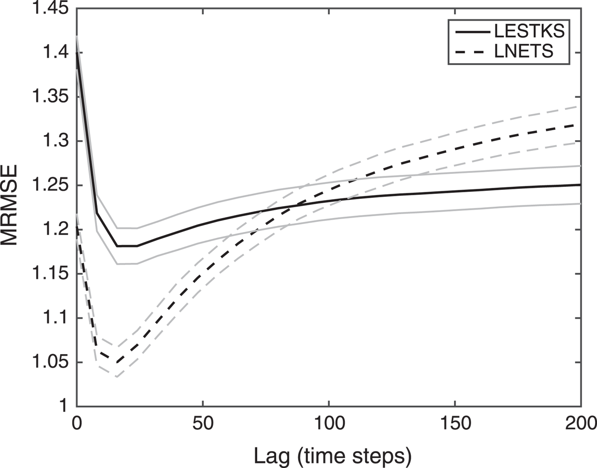
Figure 1.

If the lag is increased beyond the optimal lag, the MRMSE of both smoothers grows. For the LESTKS, the MRMSE grows slowly and approaches an asymptotic value in which the smoother provides a lower MRMSE than the filter. As explained in Nerger et al. (2014), this increase in MRMSE is caused by the model nonlinearity, while the different analysis times decorrelate for long lags without increasing the MRMSE in the case of a linear model. In comparison to the LESTKS, the MRMSE of the NETS grows faster. The MRMSE also approaches an asymptotic value for very long lags beyond the shown maximum lag of 200 time steps. However, for a lag of more than 72 time steps, the MRMSE of the smoother exceeds the MRMSE of the filter. Thus, for too long lags, the smoothing in the NETS deteriorates the filter estimate.

The difference in the dependences of the smoother performance on the lag in LESTKS and NETS is caused by the distinct update mechanisms of the analysis steps in both smoothers. In the LESTKF, the analysis covariance is determined from the forecast and observation error covariances, while the values of the observations themselves are only relevant for the update of the state estimate, i.e. the ensemble mean (Posselt et al., 2014). As described in Cosme et al. (2010), the ensemble Kalman smoothers then use the cross-covariance matrices between the current and past times. In contrast, the NETF updates both the ensemble mean and the ensemble perturbations using the observation values via their likelihoods (see Equation 4). Due to the observation errors the likelihoods can vary highly (van Leeuwen, 2009). This causes the NETF updates to be more noisy than the LESTKF updates. Thus, the direct use of the observations for filtering and smoothing limits the improvement to states at times close to the current assimilation time. Furthermore, due to the larger variability in the observations, spurious correlations over longer time spans than in the LESTKS can persist. These spurious correlations lead to the stronger increase of the RMSEs for longer lags in the NETS.

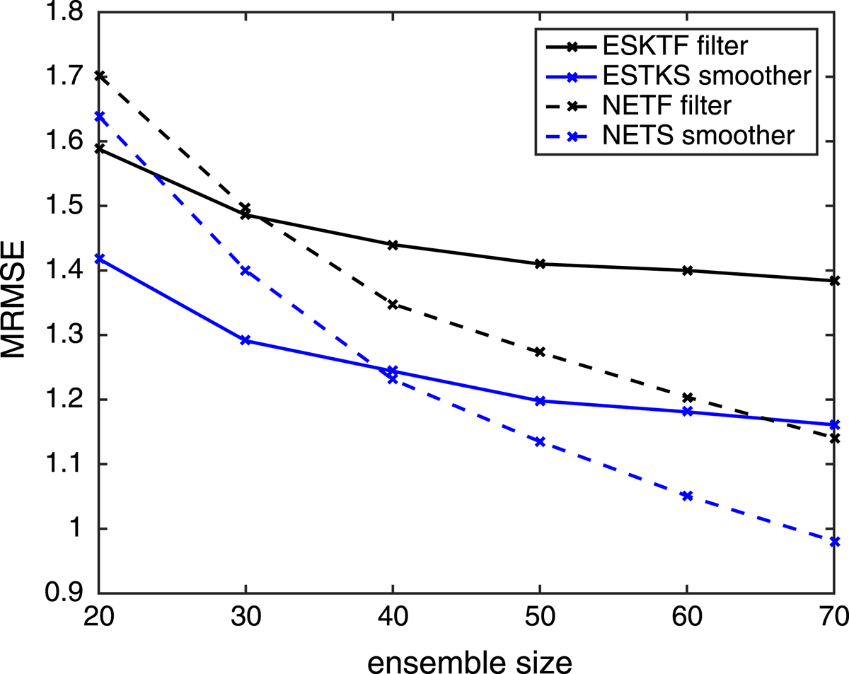
Figure 2.

The performances of the NETF and NETS depend strongly on the ensemble size, while the dependence is weaker for the LESTKF and LESTKS. Fig. 2 shows the MRMSE for different ensemble sizes between 20 and 70. For $m=20$, the MRMSE of both the NETF and NETS are higher than the MRMSE of the LESTKF and LESTKS. For $m=30$ the MRMSE of both filters are almost identical, but the LESTKS yields a lower error than the NETS. Both the NETF and NETS outperform the LESTKF and LETKS, respectively, for $m=40$ and larger. For $m=70$, the filtering in the NETF already yields a smaller MRMSE than the smoothing in LESTKS, while the NETS reduces the MRMSE below the observation error. This dependence on the ensemble size is consistent with that shown in Tödter and Ahrens (2015). ¹ Comparing the differences of the MRMSE between the smoother and filter of each method it is visible that the impact of the smoother in the LESTKS grows by a very small amount with the ensemble size. In contrast, the impact of the smoother grows significantly with the ensemble size in case of the NETS in particular for ensembles with $m\le 40$. This indicates again the important effect of sampling errors in the NETS, because the sampling errors shrink for growing ensembles.

Data assimilation setup

4.1.

To demonstrate that the introduced smoother is applicable to a realistic assimilation problem and to assess the behaviour of the NETS in a multivariate assimilation case, twin experiments with the ocean circulation model NEMO (Nucleus for European Modelling of the Ocean, Madec, 2012) are performed. As for the Lorenz-96 experiments, the NETS is compared to the square-root filter LESTKF and the smoother LESTKS. In Tödter et al. (2016) the NETF was applied to the same model configuration as used here. The computations use the same implementation of the filters and smoothers provided by PDAF (Nerger and Hiller, 2013) as used for the Lorenz-96 model. Here, only a short summary of the data assimilation setup and model configuration is presented. Additional details can be found in Tödter et al. (2016) and Yan et al. (2014).

In the experiments, a double gyre configuration of NEMO is utilised. This configuration was previously used for data assimilation experiments in several studies (Cosme et al., 2010; Yan et al., 2014; Tödter et al., 2016). In this model, the full primitive equations are solved on a regular square Arakawa C grid, using the free surface formulation. The domain extends from ${24}^{\circ }$ to ${44}^{\circ }$ in latitude, $-{60}^{\circ }$ to $-{30}^{\circ }$ in longitude and to a depth of 5054m. The configuration has $1/4^{\circ }$ horizontal resolution and 11 vertical layers. The model was configured such that the observed physical features are in good agreement to what is observed in the Gulf Stream or Kuroshio. Salinity is globally constant, so the relevant prognostic variables consist of a two-dimensional sea surface hight (SSH) fied, and the three three-dimensional fields for the horizontal velocities (U, V) and the temperature (T). For the assimilation, all variables are collected in the state vector $\mathbf{x}$ within PDAF.

The data assimilation was initialised from a 74-year model spin-up run. The following two years were used as the truth for the assimilation experiments. Assimilated were synthetic observations of temperature profiles and SSH. The temperature observations were generated by adding Gaussian random noise with a standard deviation of $0.3^{\circ }$C to the true state. The observation availability mimicked that of ARGO floats (Carval et al., 2015). As a simplification compared to the real distribution of ARGO floats, the observations were taken on a regular grid with a horizontal resolution of $3^{\circ }$. Only the upper 2000 m were observed. To simulate the motion of the floats, the observation grid was shifted by two degrees in the horizontal plane between the analysis steps. To generate the SSH observations, a random error with standard deviation of 0.06m was added to the true SSH field. This is in the same order as the error of satellite observations from Jason-1 or Envisat (see e.g. Durrant et al., 2009). The observation grid simulated satellite tracks to which the SSH from the true model trajectory was interpolated. Both SSH and T were assimilated every second day. In the second year of the experiments, the observation layout from the first year was repeated. As is typical for ocean data assimilation applications, the observations are sparse. On average, 145 SSH observations and 3128 temperature observations are assimilated at each analysis time (Tödter et al., 2016).

The initial ensemble of 120 states was generated from years 51 to 74 of the spin-up run using second-order exact sampling (Pham, 2001). The inflation factor and localisation radius were tuned to yield the minimal RMSE in the filter state estimate. All filters and smoothers were used with a horizontal localisation radius of $2.5^{\circ }$ ($\approx 250km$). In addition, the observations were weighted by a fifth-order polynomial correlation function (Eq. (4.10) of Gaspari and Cohn, 1999) depending on their distance from the analysis grid point. Inflation factors of $\mathit{\gamma }=1.02$ for the NETF/NETS and $\mathit{\gamma }=1.01$ for the LESTKF/LESTKS were used. In the experiments, both smoothers used the same observations and initial ensemble. The smoothing lag was varied between 0 (i.e. the filter) and 120 days, which results in at most 60 applications of the smoothing algorithm.

Results and discussion

4.2.

Figure 3 shows the RMSE for the SSH field for the filter and the smoother with a lag of 30 days. The RMSE of both the filter and the smoother shrinks during a spin-up phase of about 240 days. After this time, the RMSE remains constant with some short-time variability, but no trend. The NETS clearly reduces the RMSE compared to the NETF. In the first few assimilation cycles, the reduction in the error is not very large, but it increases in the following steps. After 10 analysis steps, the RMSE for the NETS is consistently smaller than for the NETF. This, shows that the spin-up phase of the smoother relative to the filter is very short compared to the filter spin-up time of about 240 days. For the other model fields, the behaviour is similar (not shown).

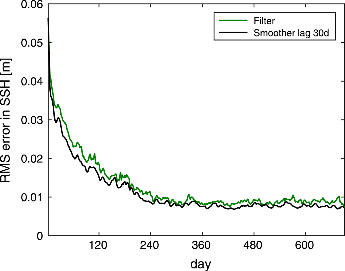
Figure 3.

In Cosme et al. (2010), it was shown that smoothing in the Kalman filter context does not only reduce the RMSE when compared to the filter, but also smoothes the trajectory such that the error remains almost constant over the whole trajectory. To this end, in Cosme et al. (2010) the measure of roughness

was introduced. A higher value of Ro indicates a higher variability in the error evolution and vice versa. Figure 4 shows the roughness of the error trajectory for all prognostic variables in dependence on the lag. The filter analysis corresponds to a lag of zero. Similar to ensemble Kalman smoother discussed by Cosme et al. (2010), the NETS reduces the roughness of the RMSE. Up to a lag of 12 days, the roughness is reduced by more than two orders of magnitude. However, a lag larger than 12 days slightly increases the roughness again, which is likely caused by the noise in the ensemble updates.

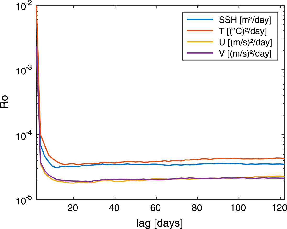
Figure 4.

To further assess the effectiveness of the smoothing in dependence of the lag, the relative improvement (Ri) is computed for all lags from 0 to 120 days according to.

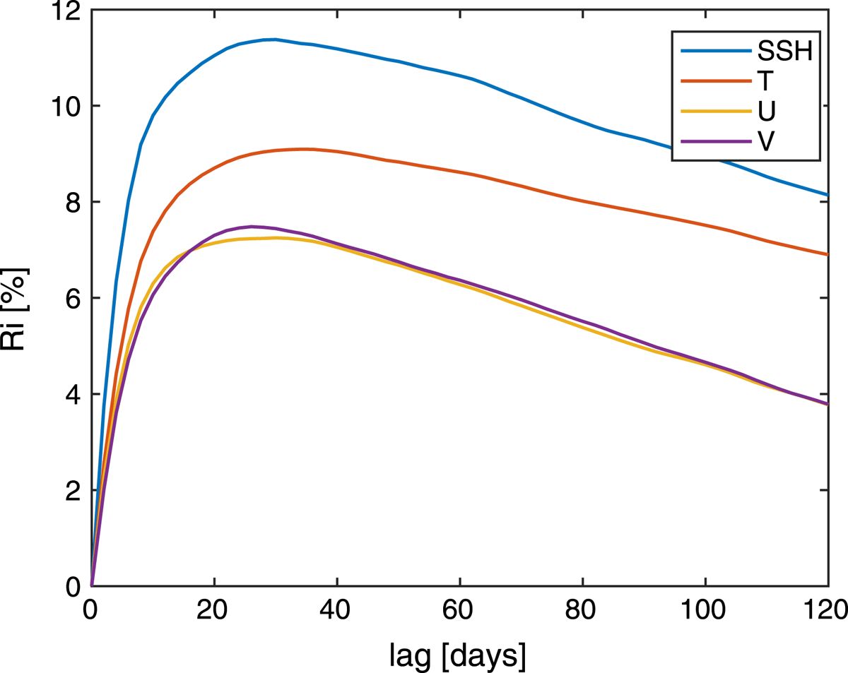
Figure 5.

Here, the MRMSE denotes the mean RMSE over the first 600 model days. Figure 5 shows that the smoother reduces the MRMSE in the smoothed ensemble for all four fields. Up to a lag of about 30 days, increasing the lag also improves the state estimate up to $11\%$ in SSH, $9\%$ in T and $7\%$ in the velocities. The reduction is strongest for the observed model fields SSH and T, but the unobserved velocities are also improved. The optimal lag is about the same if one considers the whole experimental period or if one omits the filter spin-up phase of 240 days. The relative improvement for the SSH also remains approximately unchanged with 11.1%. However, after the spin up phase, the smoothing is less effective for the temperature with an Ri of only 7.7% and a bit more effective for the velocities for which the Ri is about 8.4%.

As for the Lorenz-96 experiments, there is a lag for which the smoother yields the largest improvements. If the smoothing lag is larger than about 40 days, the Ri decreases but remains positive. Thus, the long lags do not deteriorate the filter state estimates as in the Lorenz-96 experiment. The optimal lags vary slightly for the different fields. The range of optimal lags, which is defined here as all lags whose minimal error is not more than $0.5\%$ larger than the minimum, is given in Table 1. For the NETS, the common range of optimal lags for all fields is between 24 and 36 days.

The optimal lag is significantly longer than the lag of eight days reported by Cosme et al. (2010), who used a very similar model configuration to the one assessed here. In Nerger et al. (2014), where a global ocean model with lower resolution was used, optimal lags between 40 and 170 days were found, depending on the physical fields. The long optimal lags were contributed to the low resolution of the ocean model, so that nonlinearities are weaker than in the model that was used here. In Nerger et al. (2014), the optimal lag did also vary significantly for the different fields, and hence, it was suggested to optimise the smoothing lag independently for the different model fields. This approach is not necessary here since a common optimal lag can be chosen for all fields in our experiments.

A major difference between our experiments and the experiments in Nerger et al. (2014) consists in the additional assimilation of temperature profiles. Because of these observations, the velocities in the ocean are also improved between 7–8%. This is very close to the reduction of 5–8% that was observed in Cosme et al. (2010), but is three to four times higher than in Nerger et al. (2014). The additional use of the temperature observations might be the reason why the optimal lags of the different physical fields highly overlap here in contrast to what was observed in Nerger et al. (2014).

Comparison to an ensemble Kalman smoother

4.3.

To compare the results of the NETS with an EnKF-based smoother, experiments with the same setup were performed with the LESTKS. In the same model configuration as used here, the filtering performance of the LETKF and NETF were already discussed in (Tödter et al., 2016). It was shown, that the NETF produced very similar results to the LETKF in terms of RMSE and continuous ranked probability score (CRPS, Gneiting et al., 2007).

Figure 6 shows the RMSE for the LESTKF and the LESTKS with a lag of 30 days.

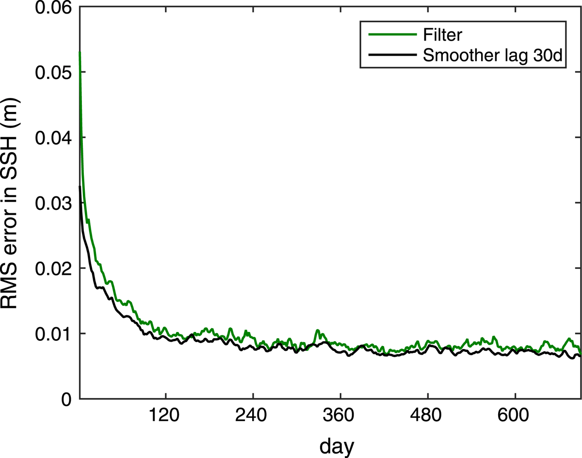
Figure 6.

The data assimilation shows a spin-up like the NETF in Fig. 3. However, the asymptotic error level is already reached after about 120 days. This shorter spin-up time was already discussed in Tödter et al. (2016). After the spin-up phase, both filters perform similarly well in the analysis. Similar to the NETS in Fig. 3, the LESTKS achieved smaller RMSEs for SSH and the other variables compared to the LESTKF. The smoother spin-up time is again only about 20 days.

The relative improvement Ri for the LESTKS is shown in Fig. 7 in analogy to Fig. 5 for the NETS. In contrast to the NETS, where all fields were improved with a similar dependence on the lag, the LESTKS exhibits a distinct behaviour for the temperature field. The Ri for SSH, U and V is reduced after smoothing for about 40 days. However, the Ri for the temperature field grows up to the maximum lag of 120 days. As mentioned above, the temperature observations also induce a positive impact for the estimation of the velocities. For the LESTKS, the impact is about 2 to 3 per cent points higher than what can be achieved by the NETS.

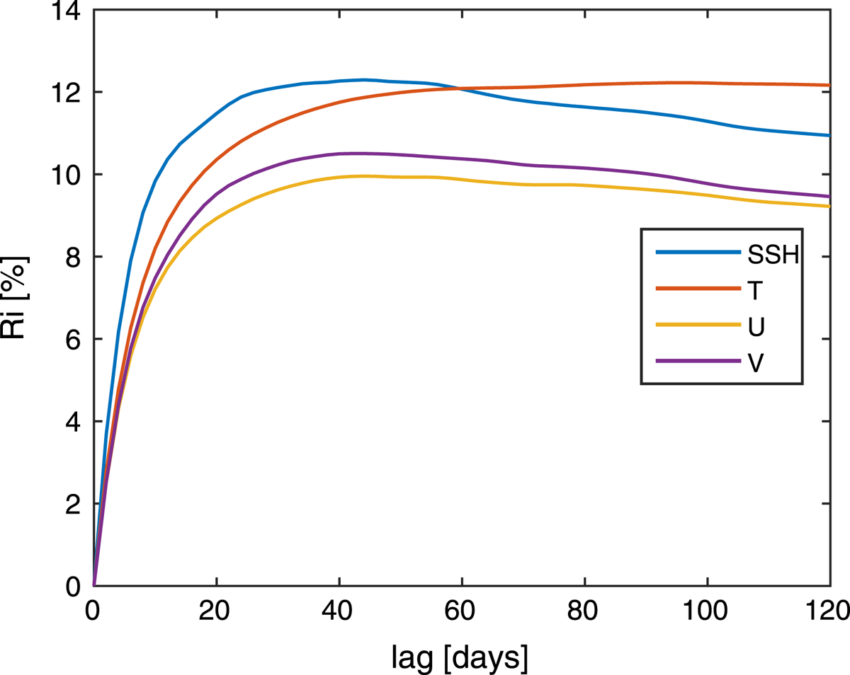
Figure 7.

The reduced sensitivity to the smoother lag in the LESTKS compared to the NETS can be attributed to the different update mechanisms in the underlying filters. As explained in Section 3, the update weights used in the filtering and smoothing in the NETF and NETS are directly computed from the likelihoods of the observations. These can vary strongly and can hence have less relevance for longer time spans and can even result in spurious temporal correlations.

Table 2 summarises the minimal values of the MRMSE and error reductions for the different fields. The error reductions for SSH in the NETS and LESTKS are very similar. Yet, the error reduction for T is larger for the LESTKS than the NETS. This also has a positive impact on the velocities. In comparison to the NETS, the minimal MRMSEs of the velocities (see Table 2) are slightly smaller for the LESTKS. This is mostly due to the faster spin-up phase in the beginning of the assimilation window but also because of the higher error reduction due to the smoothing. If one omits the filter spin-up phase of 120 days, the optimal lag is about the same as for the whole experiment. The error-reduction for the SSH also is a bit larger with 13.7%. As in the case of the NETS, and the smoothing is less effective for the temperature with an error reduction of only 11.2%. For the velocities, the error reductions are 9.7% for U and 11.0% for V.

The common optimal lag for the LESTKS is between 52 and 58 days. This is almost twice as long as for the NETS, which can also be attributed to the distinct update mechanisms.