
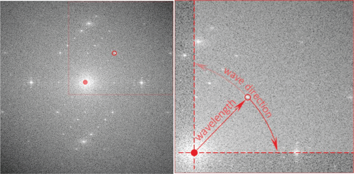
Fig. 1
Example of an FFT of a single sample of paper.
Table 1
Manufacturer, brand name, grammage, batch number of the product, and sample numbers.
| Manufacturer | Brand name, grammage and batch of the product | Sample numbers |
|---|---|---|
| Maestro | Extra, 80 g/m2, batch No. 9457 A80S | A1_1 – A1_25 |
| Maestro | Extra, 80 g/m2, batch No. 9457 A80S | A2_1 – A2_25 |
| Xerox | Premier, 80 g/m2, batch No. 003R98760 | B1_1 – B1_25 |
| NN | unknown | C1_1 – C1_10 |
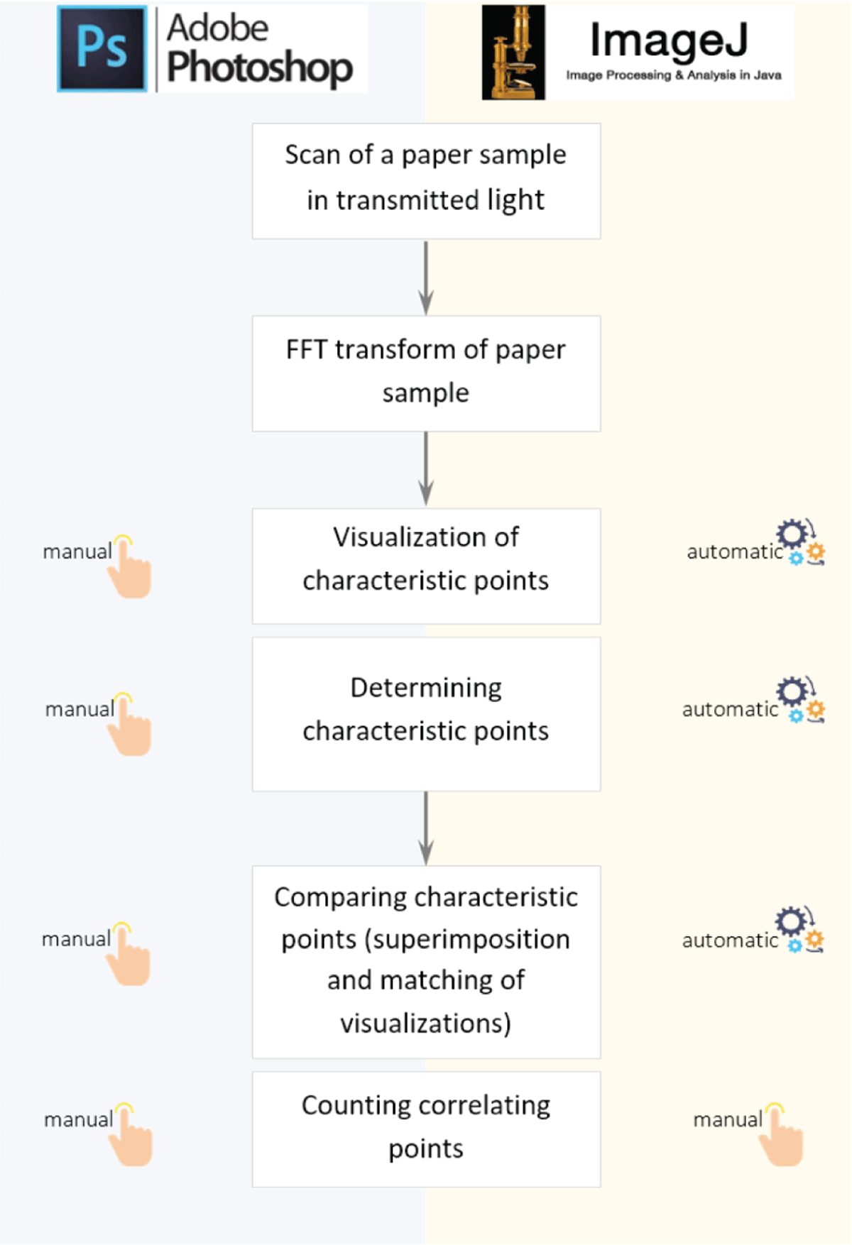
Fig. 2
Process flow of the two methods.
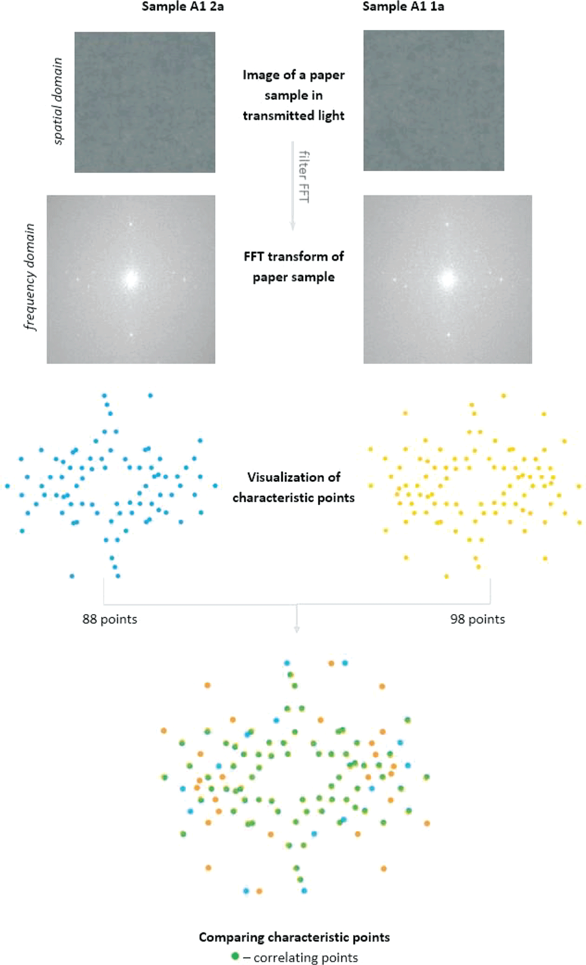
Fig. 3
Comparison of the two paper samples made using a Fast Fourier Transform (FFT).
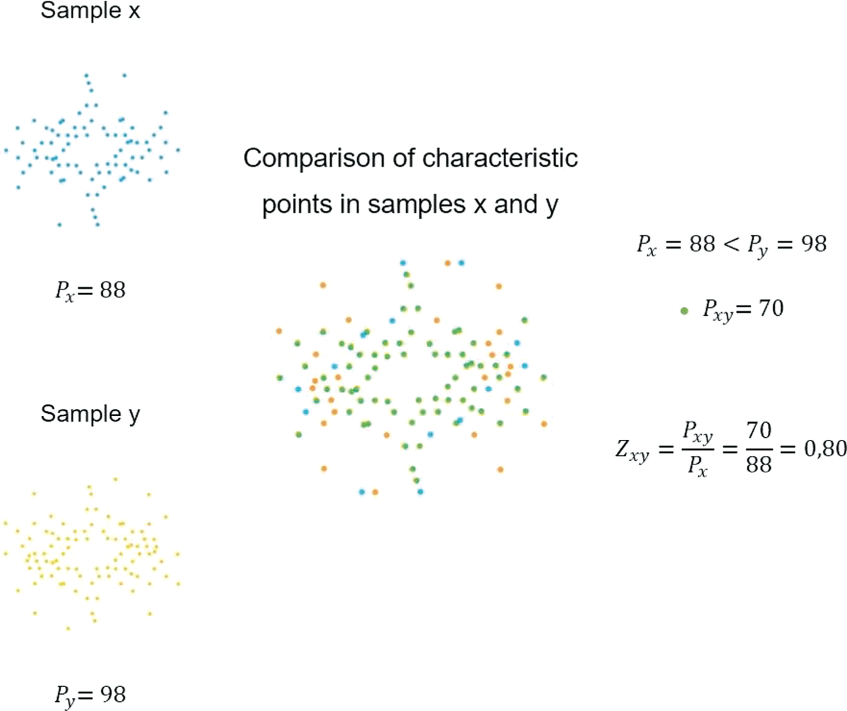
Fig. 4
Calculation of the samples’ correlation (Zxy).
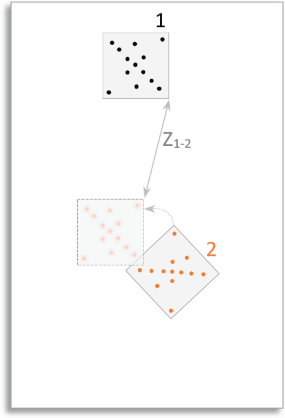
Fig. 5
Comparison of samples scanned in different orientations
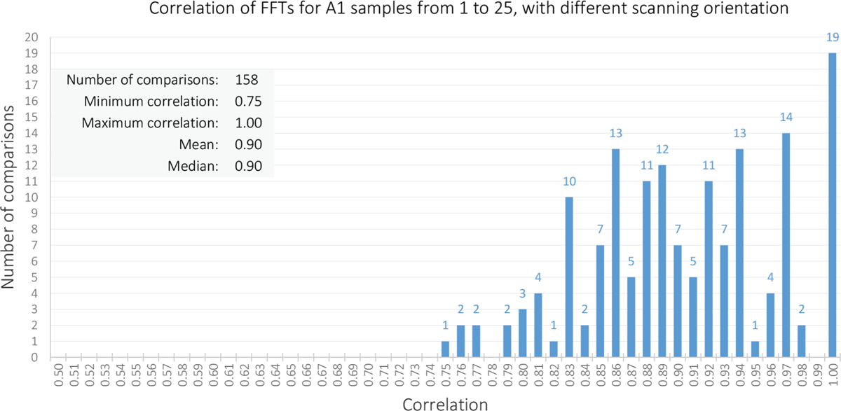
Fig. 6
Correlation of FFT samples obtained from sheets scanned with alternating orientation.
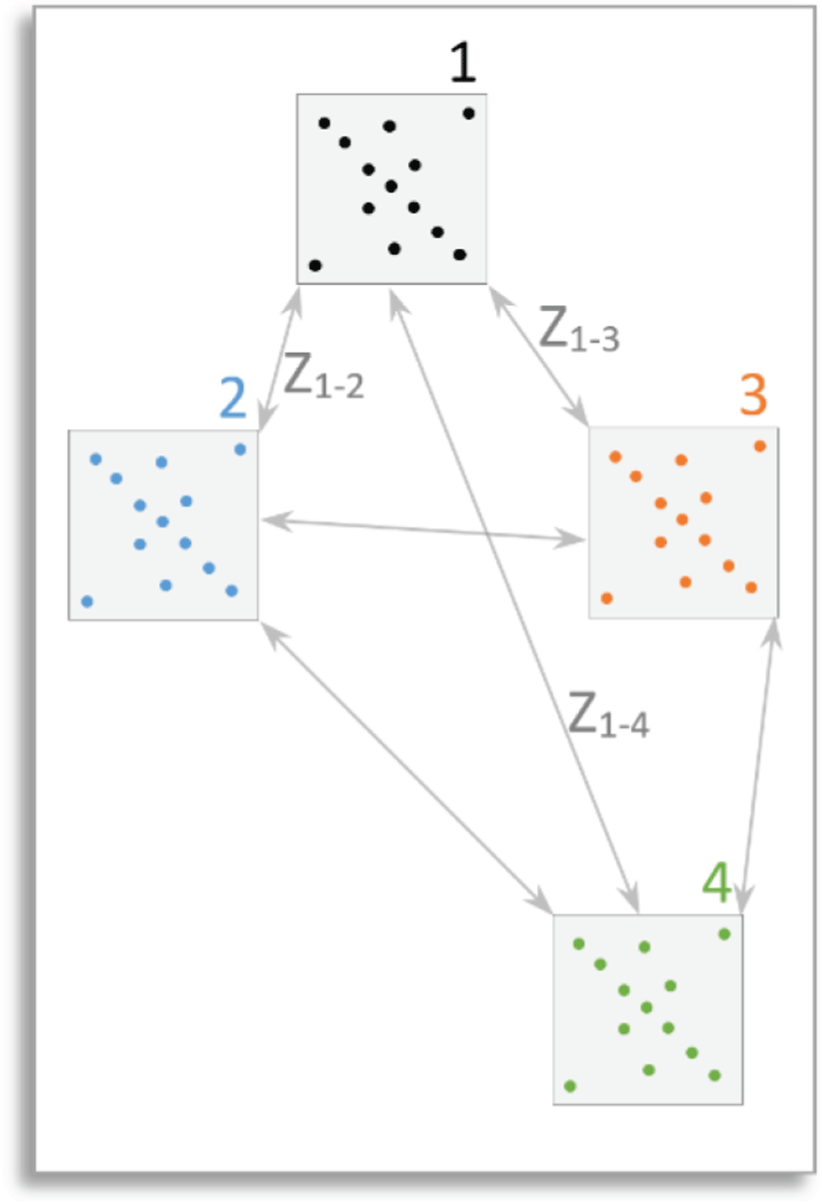
Fig. 7
Comparison of intra-source (within-sheet) samples.
Table 2
Intra-source correlation obtained when analyzing FFTs using different algorithms.
| A1 – ImageJ | A1 – Adobe Photoshop | C – ImageJ | C – Adobe Photoshop | |
|---|---|---|---|---|
| Number of comparisons | 474 | 285 | 205 | 200 |
| Minimum correlation | 0.73 | 0.68 | 0.50 | 0.60 |
| Maximum correlation | 1.00 | 1.00 | 1.00 | 1.00 |
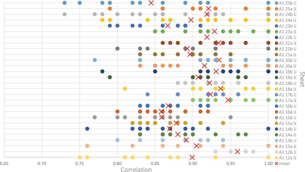
Fig. 8
Correlation ranges for comparisons of intra-source transforms (A1_12–25), using ImageJ.
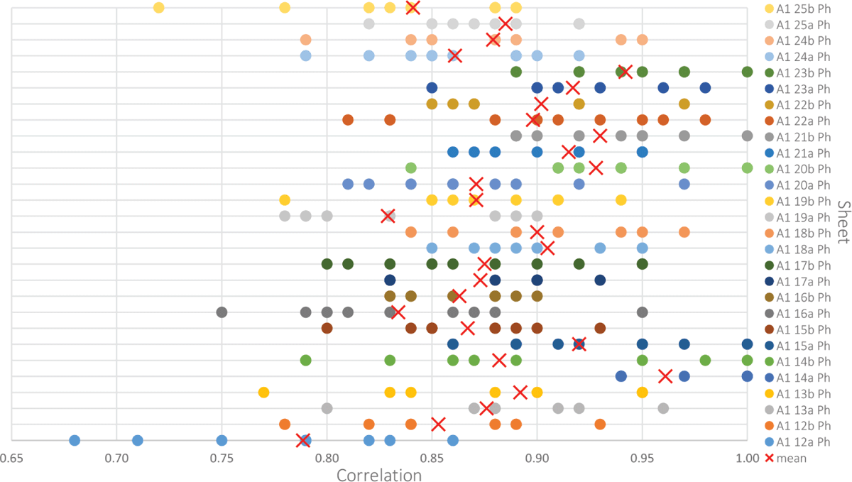
Fig. 9
Correlation ranges for comparisons of intra-source transforms (A1_12–25), using Adobe Photoshop.
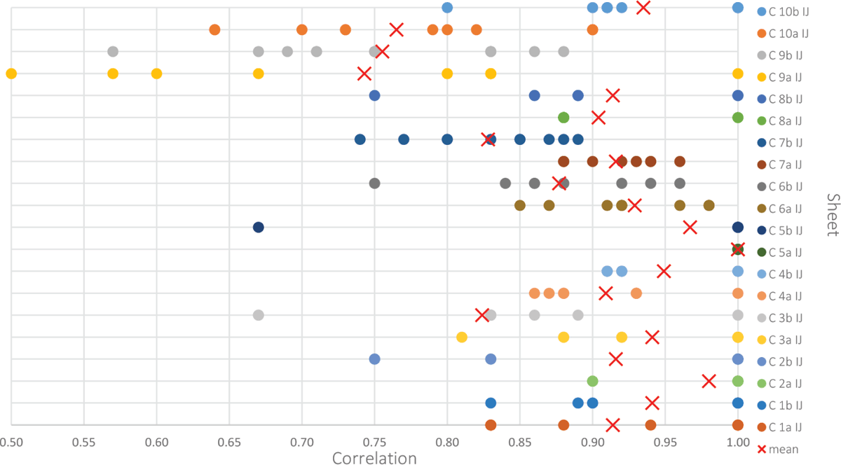
Fig. 10
Correlation ranges for comparisons of intra-source transforms (C1_1–10), using ImageJ.
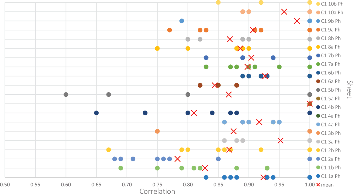
Fig. 11
Correlation ranges for comparisons of intra-source transforms (C1_1–10), using Adobe Photoshop.
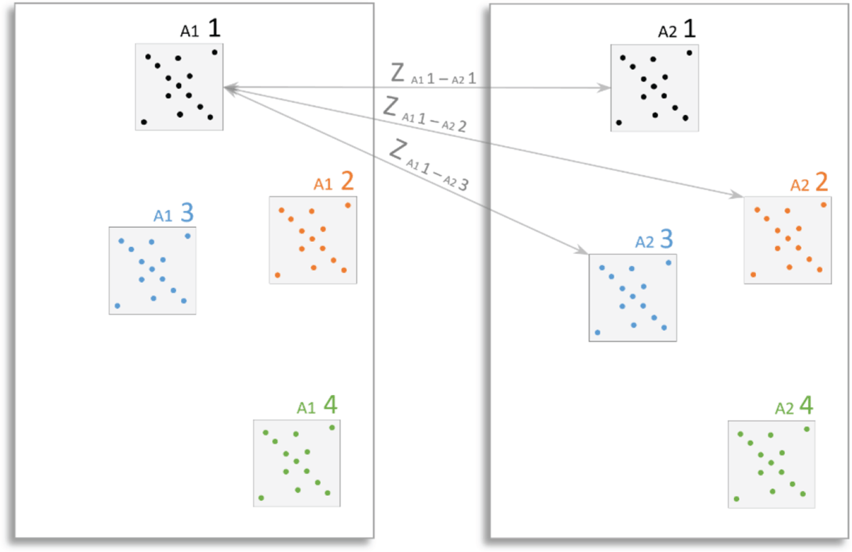
Fig. 12
Comparison of samples from two reams of the same type of paper.
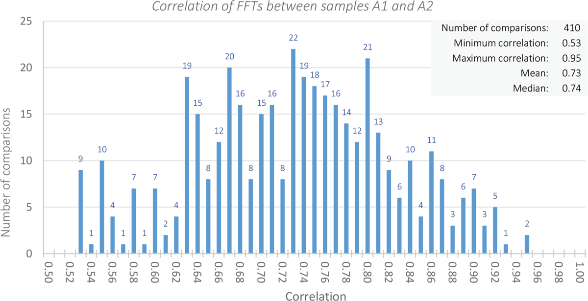
Fig. 13
Correlation of FFTs between samples A1 and A2.
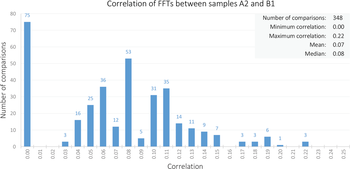
Fig. 14
Correlation of FFTs between samples A2 and B1.
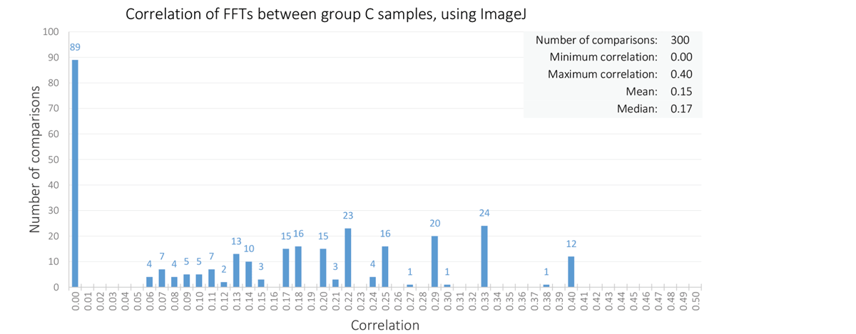
Fig. 15
Correlation of FFTs between group C samples, using ImageJ.
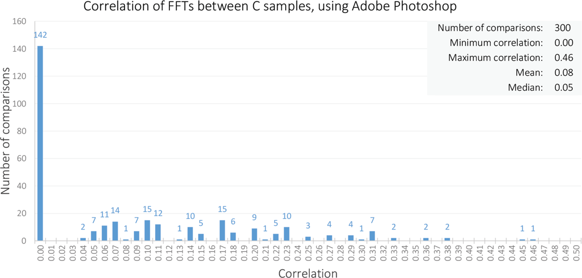
Fig. 16
Correlation of FFTs between group C samples, using Adobe Photoshop.
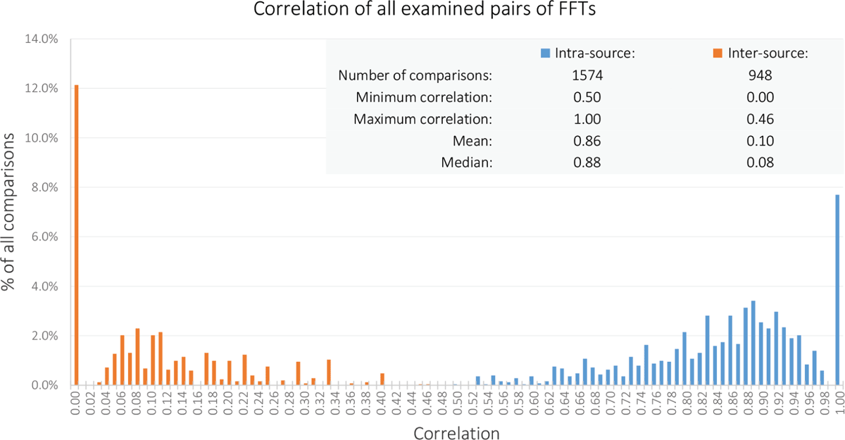
Fig. 17
Correlation of all examined pairs of FFTs.