
Introduction
This article describes a new technique which can be used for the comparison of toner. The comparison of toner is necessary in multiple topics in the field of questioned document examination, such as:
Examination of fraud; authenticity of documents
Different kinds of toners within the same page or within the same contract is an indicator for fraud
Mutual comparison of documents; are multiple documents printed on the same printer?
Linking documents to a certain printer; is this document printed on this printer?
There are lots of different ways to compare toner with the use of chemical techniques. Different techniques can be found in the literature. Reviews can be found for example in De Koeijer [1] and Partouche [2]. However, the equipment needed for these chemical analyses is often very expensive. Furthermore most analyses are semidestructive. Samples are needed of both the blank paper as well as toner. This causes damage to the original document and other traces such as fingerprints can be disturbed.
Therefore, a preliminary evaluation was performed into a non-destructive technique which measures magnetic properties of the toner. The magnetic properties of toner are already used for classification for a long time. With the use of a magneto-optical visualizer it is easy to discriminate between:
Non-magnetic toner: toner used in a dual component developing system. The toner particles are charged by triboelectrification1 and adhere to the much larger carrier beads in the developing system. The carrier beads are magnetic and can be transported easily under influence of a permanent magnet towards the drum. Near the drum the toner particles are rubbed from the carrier beads and transferred to the drum, while the carrier beads stay behind.
This type of toner is mostly used in modern color printers with chemically prepared toner particles.
Magnetic toner: toner used in a mono component developing system.
This developer consists of magnetic toner particles, so carrier beads are not necessary in the developing unit. The magnetic properties are usually caused by the magnetic pigment iron oxide (Fe3O4) in the toner particles.
This type of toner is mostly used in black and white printers with mechanically prepared toner particles.
The difference between both developers is visible with a magneto-optical visualizer, because the difference in magnetic properties between the two classes of toner is large. Non-magnetic toner shows no magnetic properties, while magnetic toner was easily visualized with such a visualizer (see Figure 3). Besides visualization it is nowadays also possible to easily perform measurements on the magnetic properties of the toner. With this preliminary evaluation we were studying if it is possible to discriminate toners within the class of magnetic toners by quantitative measurements of these properties.
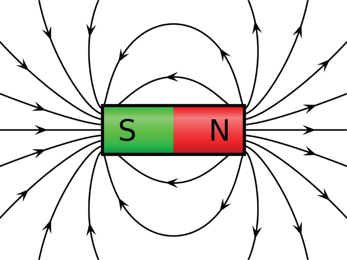
Figure 1.
Example of a magnet with a south and north pole. The lines represent the direction of the magnetic induction (B).
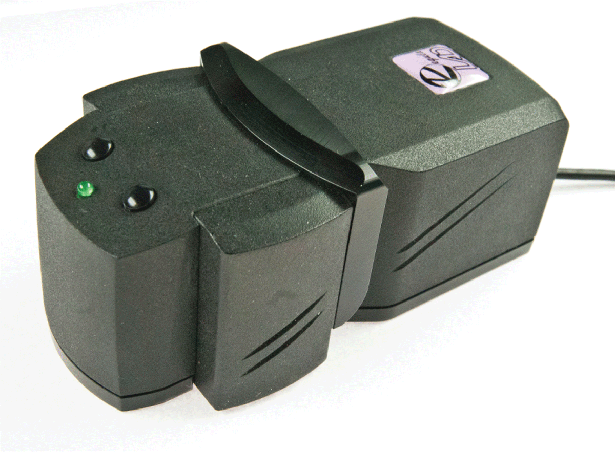
Figure 2.
Regula Magmouse Model 4197.
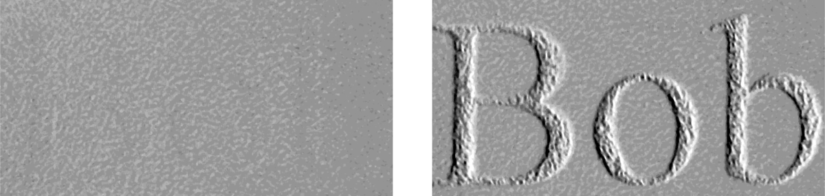
Figure 3.
Two images created with the Magmouse of the word ‘Bob’ printed with a non-magnetic toner (left) and a magnetic toner (right)
Magnetism
This theoretical part is only a very short introduction into electromagnetism in order to introduce some magnetic quantities and their units. More information can be found in many textbooks on electromagnetism.
Certain materials such as iron have magnetic properties. The strength of the magnetic properties can be expressed in the quantity of magnetic induction, B in units Tesla (T). Magnetic induction is a vector with a direction and a magnitude and describes the magnetic field strength which is present in the area surrounding an object with magnetic properties. With the measurements in this study, the magnetic induction normal to the substrate (paper) surface is measured, Bn.
The magnetic flux φ in units Weber (Wb) is another quantity which can be measured. The normal flux φ is defined as the amount of magnetic induction (‘field strength’) through a certain surface A. Only the component of magnetic induction normal to the surface is measured (Bn).
Therefore, the flux (φ) and the magnetic induction2 (Bn) are related in the following way:
1
[TeX:] \documentclass[10pt]{article} \usepackage{wasysym} \usepackage[substack]{amsmath} \usepackage{amsfonts} \usepackage{amssymb} \usepackage{amsbsy} \usepackage[mathscr]{eucal} \usepackage{mathrsfs} \usepackage{pmc} \usepackage[Euler]{upgreek} \pagestyle{empty} \oddsidemargin -1.0in \begin{document} \[ \vert\phi \vert= \int\vert B^{n}\vert dA, \] \end{document}Translated to this study: the magnetic induction (Bn) of toner was measured. Furthermore, the flux was measured through the surface area A of the measurement device. The question was whether differences can be measured in these quantities when different kinds of (magnetic) toner are used by different laser printers.
Methods and materials
Regula Magmouse
For measuring magnetic properties the Regula Magmouse Model 4197 was used, shown above.
The original purpose of the Magmouse is detection of counterfeit money, forged cheques and forged identity papers. The device visualizes magnetic properties of ink or toner, and is also able to quantitatively measure the magnetic induction and flux. The working principle is based upon an internal inductor in combination with a magneto-optical sensitive CCD sensor. More information upon the working principle can be found in Agilidi Yu [3] and the User’s Guide [4].
The device was used in combination with CADR software from Regula. The CADR software can visualize magnetic properties and can also perform measurements. The visualization option is shown in Figure 3. The Magmouse does not display the paper and toner, but only the magnetic properties. Figure 3 illustrates images of a non-magnetic toner and a magnetic toner. These pictures demonstrate that it is possible to use magnetism to discriminate between different classes of laser printers on a qualitative basis.
The question to be answered in this study was whether it is possible to use magnetism to discriminate between different laser printers on a quantitative basis. The CADR software has a special measurement module that could be used to answer this question. For every pixel of the sensor, the magnetic induction in the normal direction was measured. The results were plotted in a histogram together with the calculated flux3, see equation (1). The x-axis of the histogram describes the strength of the magnetic induction (Bn) in mT and the y-axis describes the number of pixels N (logarithmic scale, 10log(N)) associated with the corresponding strength of magnetic induction. The sign of the numbers on the x-axis (the magnetic induction) is related to the direction of the magnetic induction; the direction of the magnetic induction is up or down. Most materials show symmetric behavior in both directions. The total number of pixels of the Magmouse sensor is 1024 x 1280 = 1310720 pixels, corresponding to 106.11751.
As an example, the measurements of the samples in Figure 3 are shown in the histogram in Figure 4. Again there is a major difference between a non-magnetic toner (above) and a magnetic toner (below).
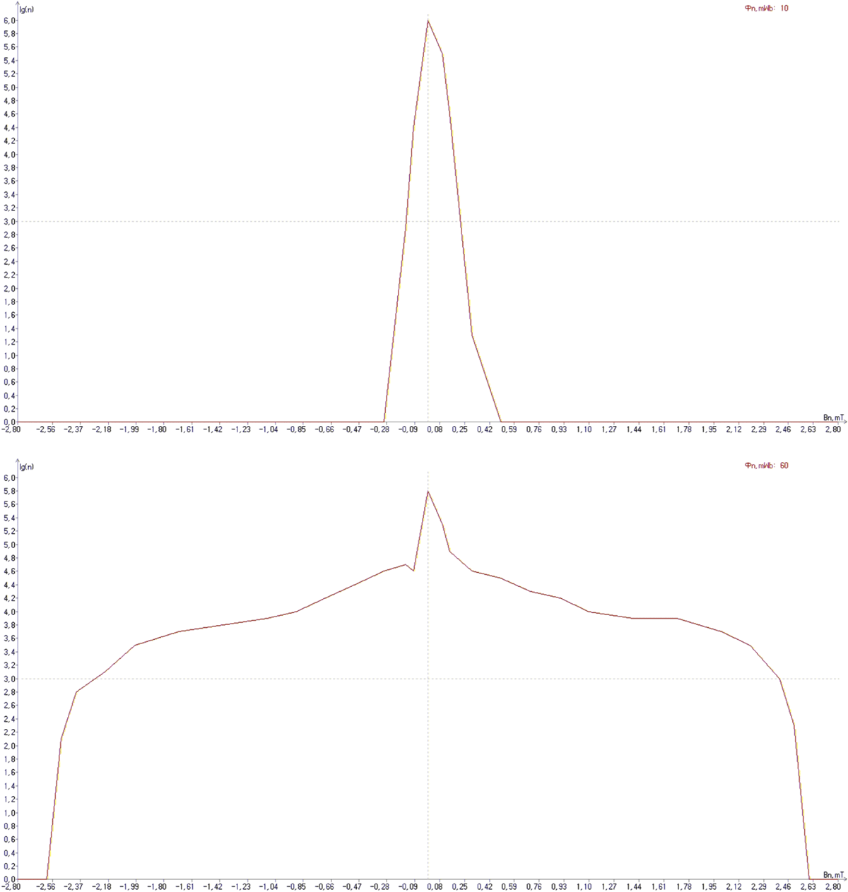
Figure 4.
Histogram of magnetic induction of a non-magnetic toner (above) and a magnetic toner (below). The x-axis describes the strength of the magnetic induction in mT and the y-axis describe the number of pixels N (logarithmic scale, 10log(N)).
As can be seen in Figure 4, no magnetic induction (dashed line: Bn = 0) is measured for most pixels of the non-magnetic toner sample (N ≈ 106) resulting in a relatively small peak area in the histogram above and a measured flux of 10 nWb. In the magnetic sample, a lot more magnetic induction is measured. This results in a broad histogram and c onsequently a bigger peak area and a higher flux (60 nWb).4
Print samples
This study used 72 print samples from 19 different laser printers which all use magnetic toner, see Appendix A for a list of used printers and number of samples. For each sample the flux and magnetic induction of the toner was measured on several locations on one page with the Regula Magmouse Model 4197. The samples were already collected for different research projects and not specially designed for this study.
The samples were documents with text only (see Appendix B for an image), printed on the same type of paper. The samples consisted of black text only in different fonts. The word ‘Bob’ is chosen to perform the measurements. For all three fonts, the word could be captured by a measurement of approximately 500 by 250 pixels of the Magmouse. The three fonts were: Times New Roman (12pt); Arial (11pt); and Calibri (12pt).
Measurements
The measurements were done according to a clear script to make sure the measurements were done without any variation in the measurement procedures. For example, for each measurement the same location of the sensor was used to avoid any variation within the measurement device.
Furthermore, repeatability and reproducibility of the Magmouse were studied. The repeatability is characterized by the same conditions (e.g. location in the lab, measuring area on the sensor of the Magmouse), while with reproducibility the effects of each condition are examined by changing only one condition at a time. Of course the same sample and word was measured every time: ‘Bob’, Times New Roman, 12pt printed on a HP LaserJet P1006.
In this study the following conditions were considered:
Location in the lab
Measuring area on the sensor of the Magmouse
Location in the lab
In the questioned document examination laboratory many tables, chairs and electrical equipment are present. Some parts of the tables, chairs and electrical equipment influence the magnetic field in the laboratory, so the location of the measurements can influence the results.
The standard location was on a small wooden table. For the test on reproducibility ten different locations were chosen: three different locations in the laboratory on the small wooden table (the table was replaced every time), three locations on the floor, three locations on a table with metal parts and one location on a marble table (see Figure 5).
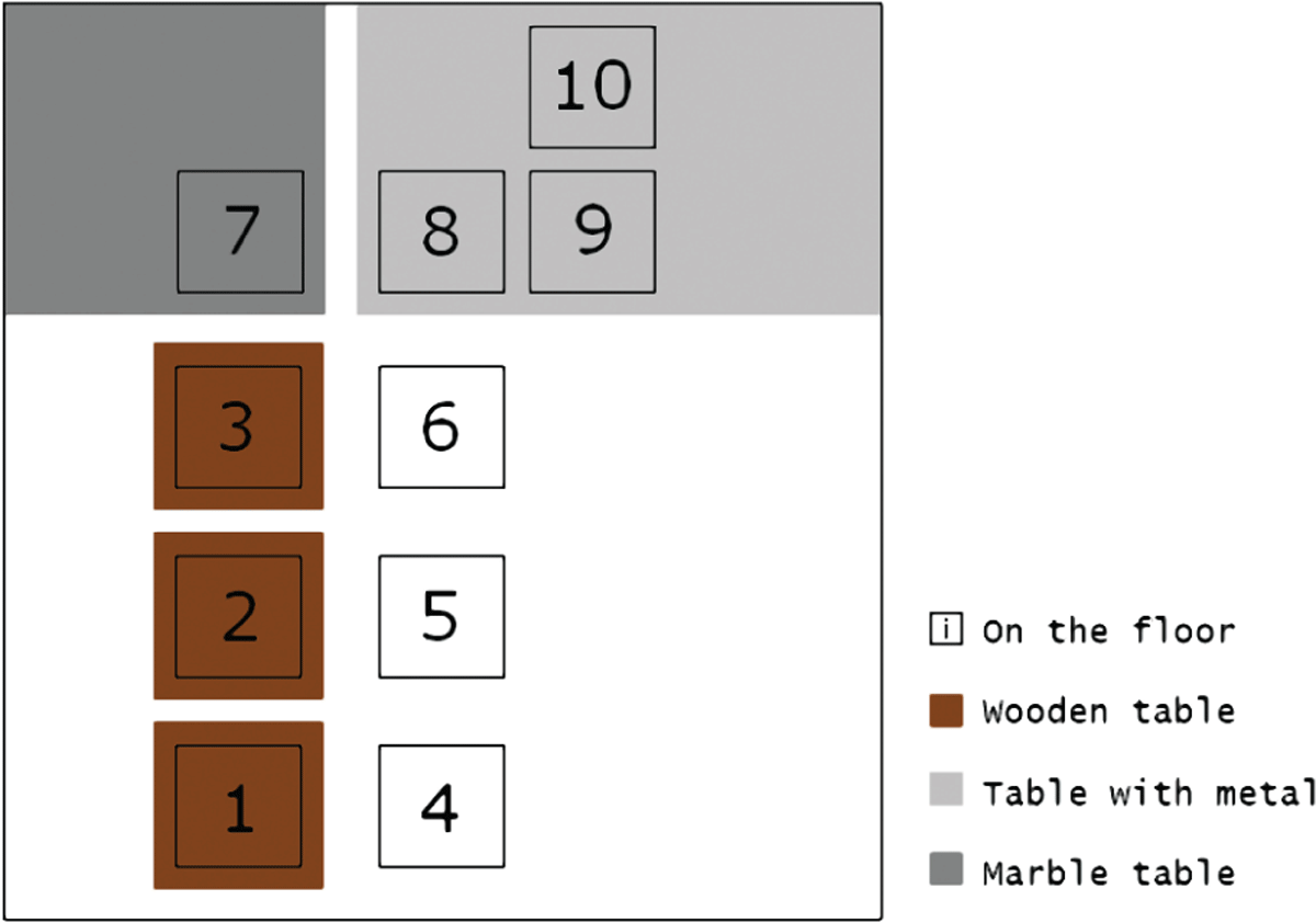
Figure 5.
Ten different locations in the laboratory.
Measuring area on the sensor of the Magmouse
The measuring area is a magneto-optical sensitive element at the bottom of the Magmouse. The element is 14x18mm, which corresponds with 1024x1280 pixels. The areas which were measured are smaller than the sensitive element, approximately 500 x 250 pixels. So, it was necessary to know whether the location in the measuring area could influence the results. For that reason ten different locations on the sensor were chosen.
Likelihood-ratio framework
As in many sciences, statistics are also used in forensic sciences. There is a distinction between descriptive statistics and inferential statistics. The latter is used to draw conclusions from data, and that is exactly what is needed in forensic sciences. The likelihood-ratio framework is a part of inferential statistics. In this section the general theory is applied to questioned document examination with respect to the magnetic properties of toner particles. For all calculations and plots, the scientific software MATLAB5 was used.
Hypotheses
In questioned document examination often two documents are compared. The question usually is whether the documents originate from the same printer. For that reason the hypotheses can be formulated in the following way:
H0 Documents A and B originate from the same printer (null hypothesis)
H1 Documents A and B originate from different printers (alternative hypothesis)
Score
In this study the magnetism of toner particles was measured. In comparing samples A and B, it was necessary to quantify the difference between both samples. There are several possibilities for this quantification. In this study, ten different options were used, that can be subdivided in three sets: distance measures in a finite vector space, distance measures in a function space and correlation measures. To reduce the amount of mathematics in this article, this will not be discussed in detail. This information can be found in Mieremet [6]. The quantification of the difference in magnetism between two samples A and B is called the ‘score’ in this article.
Within-and-between variation
In order to interpret the score, it is necessary to known how often this score occurs:
when two documents are printed with the same printer (within variation), and
when two documents are printed with different printers (between variation).
How often a certain score occurs when two documents are printed with the same printer can be determined by a so-called “within variation” curve. Such a curve is constructed by performing lots of measurements on different samples printed with the same printers. Subsequently, samples printed with the same printer were compared to each other and the within scores were determined. The next step was to plot these scores in a histogram to see how often a certain score occurs.
The contour of such a histogram was estimated by the estimation of a probability density function. However, this last step is more a mathematical problem which will not be further discussed in this article (for more information, see Mieremet [6]).
How often a certain score occurs when two documents are printed with different printer can be determined by a socalled “between variation” curve. Such a curve was constructed by performing lots of measurements on different samples printed with different printers. Subsequently, samples printed with a different printer were compared to each other and the between scores were determined. The next step was to plot these scores in a histogram to see how often a certain score occurs.
Again, the contour of such a histogram was estimated by the estimation of a probability density function (for more information, see Mieremet [6]).
Likelihood ratio
The interpretation of the score was based upon the within-variation and between-variation curves, described above. The evidential power was expressed as the likelihood ratio (LR).
The LR is given by the quotient of the probability that a certain score occurs given that both documents are printed by the same printer over the probability that this score occurs given that both documents are printed by different printers.
This results in the fact that the LR then must be equal to the quotient of the within-curve over the between-curve, expressed in a formula:
2
[TeX:] \documentclass[10pt]{article} \usepackage{wasysym} \usepackage[substack]{amsmath} \usepackage{amsfonts} \usepackage{amssymb} \usepackage{amsbsy} \usepackage[mathscr]{eucal} \usepackage{mathrsfs} \usepackage{pmc} \usepackage[Euler]{upgreek} \pagestyle{empty} \oddsidemargin -1.0in \begin{document} \[ LR(score)= \frac {P(score\ \vert H_{0})} {{P(score \vert H_{1})}} \approx \frac{within\ variation\ (score)} {between\ variation\ (score)} \] \end{document}Interpretation of LR
The best way to explain the interpretation of the LR is with help of two examples (fictitious numbers are used for these examples).
Example #1
A threatening letter (printed by a laser printer) has been received by the president. An investigation has started and a suspect is found. After a search the police found a laser printer in the suspect’s house. A test print is made with the laser printer and compared to the threatening letter. The comparison results in a score of 3.1. From the within- and between-variation curves, it is calculated that this results in a LR of 16. A LR bigger than one means that the null hypothesis is in favor over the alternative hypothesis.
This means that whatever you believed before this evidence was presented, you should now be 16 times more likely than before to believe that the threatening letter and the test print are produced by the same printer.
Example #2
Two companies signed a contract (printed by a laser printer) in duplicate. One company claims that the other company altered the contract, but cannot show their copy due to a bad administration. The word ‘the’ at the beginning of the contract is compared with the word ‘the’ in the questioned section of the contract. The comparison results in a score of 22.3. This results in a LR of 0.005 (1/200). This LR is smaller than one, which puts the alternative hypothesis in favor over the null hypothesis. This means that whatever you believed before this evidence was presented, you should now be 200 times more likely than before to believe that the contract is printed by two different printers. Compared to the first example the evidential power is now much larger and in favor of the alternative hypothesis.
The likelihood ratio thus gives the evidential power in favor of one of the hypothesis.
Results
Repeatability and reproducibility of the Magmouse
Repeatability
The repeatability test consisted of 30 measurements on a wooden table (location 2, Figure 5) in the upper left corner of the measuring area of the CCD chip for a duration of 16 days. The results are shown in the left graph of Figure 7 (mean = 60.4mT and the standard deviation = 2.4mT).
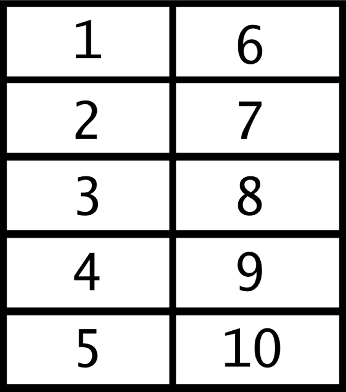
Figure 6.
Ten different measuring areas on the sensor of the Magmouse.
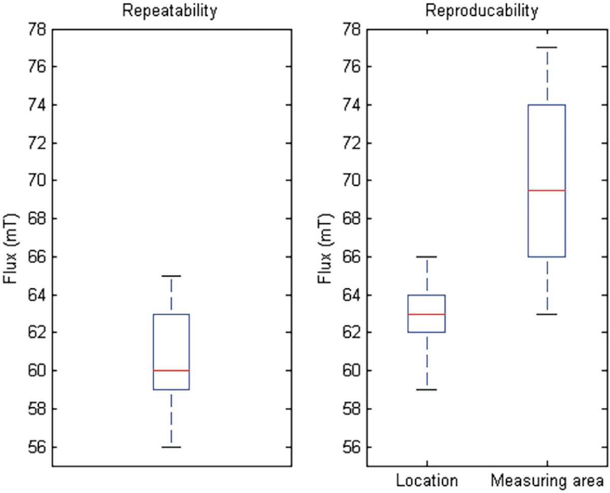
Figure 7.
Boxplot of the variation in flux.
Reproducibility
The reproducibility consisted of 10 measurements for each condition (e.g. location in the lab, location on the sensor). The right graph in Figure 7 shows two boxplots that represent the variation when the location in the lab is changed and the variation when the location on the measurement sensor is changed. A slightly higher mean (62.9mT) was calculated and a similar standard deviation (2.1mT) for the changed location, but the difference was much bigger when the measuring area was changed. The mean was calculated to be 69.6mT with a standard deviation of 4.6mT.
In a comparative evaluation, the mean is less important than the standard deviation. For that reason, it was concluded that the changing the location will not influence the results, but changing the measuring area will influence the results.
All measurements for the rest of the study were done at location 2 in the laboratory and at the top left corner in the measuring area of the CCD sensor.
Scoring methods
Ten different scoring algorithms were tested on the measured data. To calculate the scores, the data of the measured magnetic induction histograms was used, shown in Figure 4. This data is more comprehensive than the single number given by the flux. Since the flux is calculated from the magnetic induction, it is nonsensical to use both in the scoring. The best scoring algorithm for this study, based upon the log-likelihood-ratio-cost (Morrison [5]), is the 1-norm distance score, also known as the Manhattan distance score. This score can be visualized as the total area between the two histogram curves of two measurements. Figure 8 shows the measurement of a sample printed with a HP LaserJet 2200 (red curve) and HP LaserJet 4100 (blue curve). The calculated distance score is the total area between the two curves. The details of the calculations are shown in Appendix C.
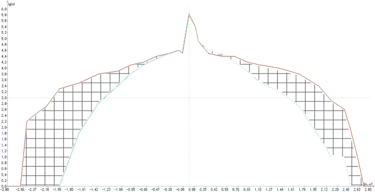
Figure 8.
The measurement of a sample printed with a HP LaserJet 2200 (red curve) and HP LaserJet 4100 (blue curve). The x-axis describes the strength of the magnetic induction in mT and the y-axis describe the number of pixels N (logarithmic scale, 10log(N)). The squared area is a visualization of the calculated 1-norm distance score (Manhattan distance score).
The remainder of this article only shows results of the 1-norm distance score. Details and results on other scoring algorithms can be found in Mieremet [6].
Within-variation and between-variation
The smaller the distance score, the more correspondence in magnetic induction between two samples. Therefore, one would expect that samples originating from the same printer (within-variation) result in low scores. In order for this method to be successful for this application, scores of samples originating from different printers (between variation) should be high. The outcome of the within-variation and betweenvariation scores is shown below in Figure 9. This shows the results of 105 scores comparing samples from the same printer (within-variation) and 2451 scores comparing samples from different printers (between-variation). The details can be found in Appendix C.
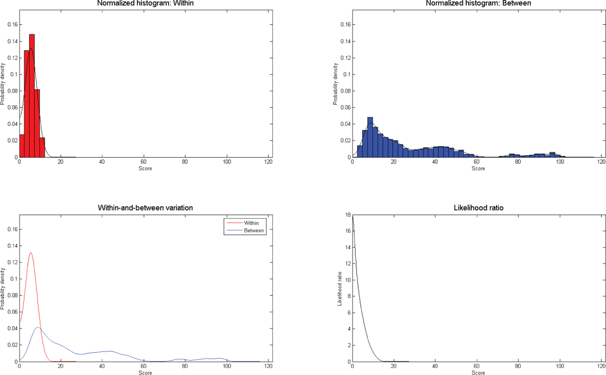
Figure 9.
Top left shows the within-variation histogram; top right shows the between-variation histogram; Bottom left shows the probability density curves (red within-variation / blue between-variation); Bottom right shows the LR as function of the score.
In Figure 9, the LR is shown in a linear scale. To see more detail, especially in the LR values smaller than 1, a logarithmic scale for the LR value can be used. This is visualized in Figure 10. The intersecting point with a LR value of 1 is at a distance score of 10. A distance score lower than 10 gives support the null hypothesis (same printer) while distance scores above 10 give support to the alternative hypothesis (different printer). In Figure 10, it is clear to see that the evidential power for supporting the alternative hypothesis (different printer), can be much larger than the evidential power for supporting the null hypothesis (same printer).
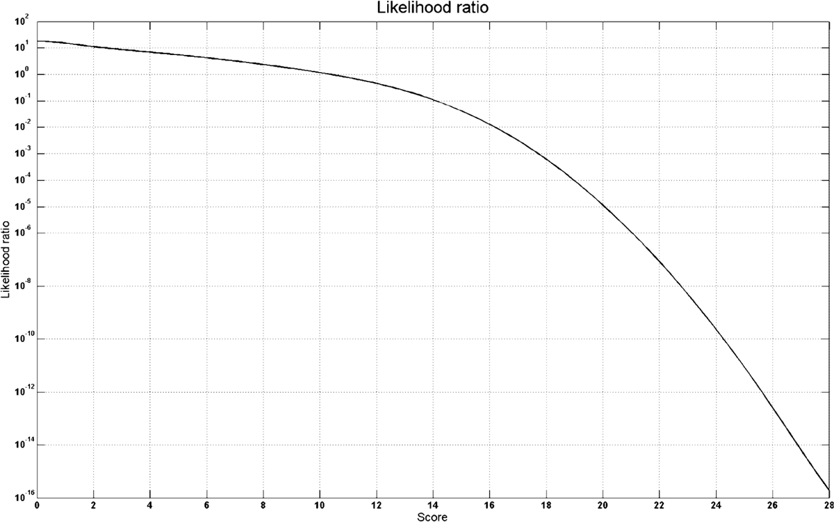
Figure 10.
LR values plotted on a logarithmic scale.
In other words, if there is a big difference in magnetic induction (high score) between two samples, this result provides a lot of support that different printers are used.
Discussion
Quality of the database
The quantity of samples that were used in this study is 72 prints from 19 different laser printers from 3 different brands. This size is large enough for a preliminary investigation, but for a proper representation more prints from additional printers would be needed. Therefore, these results and evidential powers are not to be used in regular casework.
Ideally, a lab should have a database of print samples representative of the printers used in the relevant population. So for the Netherlands, a database of print samples representing the market distribution of printers in the Netherlands should be constructed.
Comparing different but comparable fonts
In the results shown above, the measurements were scored by comparing the word “Bob” in three different fonts on sample A with the word “Bob” in three different fonts on sample B. However, the same font was compared to the same font and no ‘mixed font’ comparison was done in the previous results. It is likely that the magnetic induction measured from a sample is depended on font, since a different font will be printed with a different amount of toner. A different amount of toner will probably result in a different magnetic induction. Nevertheless, the three fonts chosen for this study showed a corresponding variation in flux, see Figure 11.
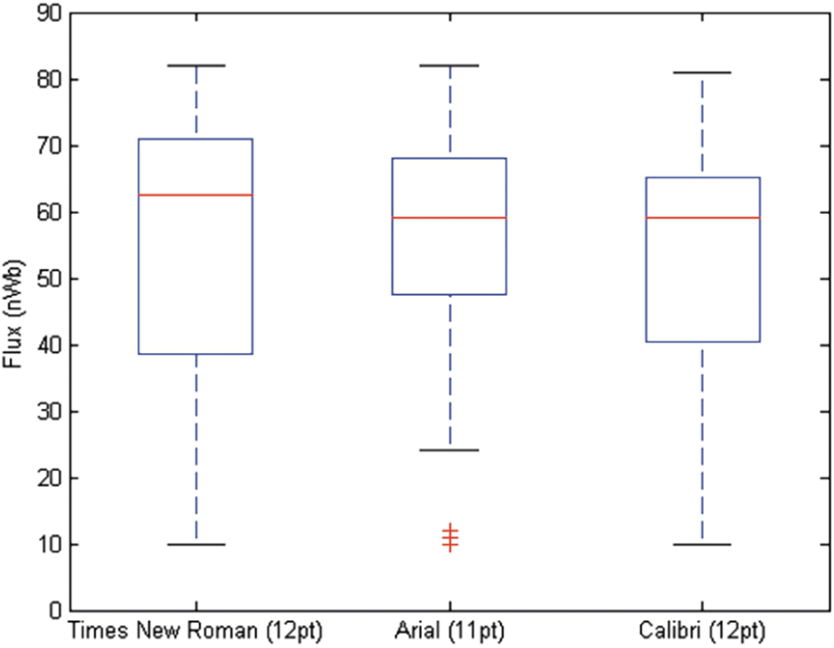
Figure 11.
Boxplots of the variation in flux of the word “Bob” in three different fonts.
The central mark is the median, the edges of the box are the 25th and 75th percentiles, the whiskers extend to the most extreme data points not considered outliers, and outliers are plotted individually.
Evidential power
The evidential power supporting the null hypothesis (same printer) has the order of magnitude 10 (depending on the score). Compared to evidential power with DNA matches, this is low. However, scientists should realize that the evidential power is related to the alternative hypothesis. In this study, the alternative hypothesis is limited to different printers also using magnetic toner. In other words, a printer is not compared with every other possible printer. Inkjet printers, printers using non-magnetic toners, dot-matrix printers, thermal printers, etc. are already excluded. If these excluded printers are also taken into account in the alternative hypothesis, the evidential power will rise substantially.6
The evidential power supporting the alternative hypothesis can become very large (for large scores). Consequently, this method could provide strong evidence for fraud when multiple printers are used on the same document.
Recommendations
In this preliminary evaluation, the influence of paper and time was not studied thoroughly. It is not known whether the magnetic properties of a print decreases after some period of time. Probably the magnetic properties of the toner material itself will not be effected by time. However, it is possible that the amount of toner particles on the print will change over time due to scraping off the toner (unintentionally or intentionally). The hypothesis is that the influence of paper is small, especially limited to normal multifunctional printing paper. The adhesion of toner particles will differ between different papers, but the influence on the magnetic properties is probably low.
However, it is very important to investigate these possible influences because questioned document examiners may deal with older documents and different kinds of paper.
The amount of toner is also important when performing measurements on different fonts, font sizes or different words. With image processing software, it is quite easy to measure the area of toner on a surface. Maybe it is possible to incorporate the area of toner into the comparison to compensate for different areas.
Conclusion
This study demonstrates that this technology has the potential to discriminate between different printers. The Magmouse was easy to operate and measurements can be done quickly without contaminating, damaging or destroying other traces on the document. However, the range of application is limited to documents printed with magnetic single-component toner, which (in the Netherlands) is a minority of the printers. More research is necessary before this technology can be used in casework.
Appendices
Appendix A: Table with used printers and samples
Table A-1
Used printers during this study with corresponding sample numbers.
| Sample ID | PrinterID | Brand | Type |
|---|---|---|---|
| 1 | 1 | Canon | ImageClass MF4770n |
| 2 | 1 | Canon | ImageClass MF4770n |
| 3 | 1 | Canon | ImageClass MF4770n |
| 4 | 1 | Canon | ImageClass MF4770n |
| 5 | 2 | Dell | Laserprinter 1700 |
| 6 | 2 | Dell | Laserprinter 1700 |
| 7 | 2 | Dell | Laserprinter 1700 |
| 8 | 2 | Dell | Laserprinter 1700 |
| 9 | 3 | HP | LaserJet 1018 |
| 10 | 3 | HP | LaserJet 1018 |
| 11 | 3 | HP | LaserJet 1018 |
| 12 | 3 | HP | LaserJet 1018 |
| 13 | 4 | HP | LaserJet 2200 (series PCL 5) |
| 14 | 4 | HP | LaserJet 2200 (series PCL 5) |
| 15 | 4 | HP | LaserJet 2200 (series PCL 5) |
| 16 | 4 | HP | LaserJet 2200 (series PCL 5) |
| 17 | 5 | HP | LaserJet 4100 (series PCL) |
| 18 | 5 | HP | LaserJet 4100 (series PCL) |
| 19 | 5 | HP | LaserJet 4100 (series PCL) |
| 20 | 5 | HP | LaserJet 4100 (series PCL) |
| 21 | 6 | HP | LaserJet 4L |
| 22 | 6 | HP | LaserJet 4L |
| 23 | 6 | HP | LaserJet 4L |
| 24 | 6 | HP | LaserJet 4L |
| 25 | 7 | HP | LaserJet 6L |
| 26 | 7 | HP | LaserJet 6L |
| 27 | 7 | HP | LaserJet 6L |
| 28 | 7 | HP | LaserJet 6L |
| 29 | 8 | HP | LaserJet 5P |
| 30 | 8 | HP | LaserJet 5P |
| 31 | 8 | HP | LaserJet 5P |
| 32 | 8 | HP | LaserJet 5P |
| 33 | 9 | HP | LaserJet 4L |
| 34 | 9 | HP | LaserJet 4L |
| 35 | 9 | HP | LaserJet 4L |
| 36 | 9 | HP | LaserJet 4L |
| 37 | 10 | HP | LaserJet Pro 400 M401dw |
| 38 | 10 | HP | LaserJet Pro 400 M401dw |
| 39 | 10 | HP | LaserJet Pro 400 M401dw |
| 40 | 10 | HP | LaserJet Pro 400 M401dw |
| 41 | 11 | HP | LaserJet 600 M602 |
| 42 | 11 | HP | LaserJet 600 M602 |
| 43 | 11 | HP | LaserJet 600 M602 |
| 44 | 11 | HP | LaserJet 600 M602 |
| 45 | 12 | HP | LaserJet P1006 |
| 46 | 12 | HP | LaserJet P1006 |
| 47 | 12 | HP | LaserJet P1006 |
| 48 | 12 | HP | LaserJet P1006 |
| 49 | 13 | HP | LaserJet 1022nw |
| 50 | 13 | HP | LaserJet 1022nw |
| 51 | 13 | HP | LaserJet 1022nw |
| 52 | 13 | HP | LaserJet 1022nw |
| 53 | 14 | HP | LaserJet P2015dn |
| 54 | 14 | HP | LaserJet P2015dn |
| 55 | 14 | HP | LaserJet P2015dn |
| 56 | 14 | HP | LaserJet P2015dn |
| 57 | 15 | HP | LaserJet P2035 |
| 58 | 15 | HP | LaserJet P2035 |
| 59 | 15 | HP | LaserJet P2035 |
| 60 | 15 | HP | LaserJet P2035 |
| 61 | 16 | HP | LaserJet P2055dn |
| 62 | 16 | HP | LaserJet P2055dn |
| 63 | 16 | HP | LaserJet P2055dn |
| 64 | 17 | HP | LaserJet 4015 |
| 65 | 18 | HP | LaserJet 4250 TN |
| 66 | 18 | HP | LaserJet 4250 TN |
| 67 | 18 | HP | LaserJet 4250 TN |
| 68 | 18 | HP | LaserJet 4250 TN |
| 69 | 19 | HP | LaserJet 4250dtn |
| 70 | 19 | HP | LaserJet 4250dtn |
| 71 | 19 | HP | LaserJet 4250dtn |
| 72 | 19 | HP | LaserJet 4250dtn |
Appendix B: Image of sample page (scaled down from A4 size)
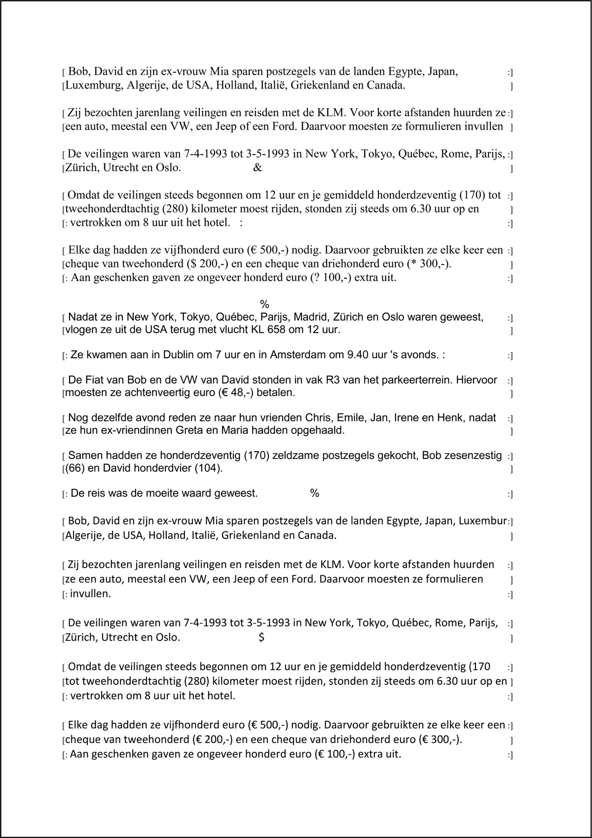
Figure B-1.
Image of sample page. Original sample page was A4 size.
Appendix C: Processing of the measurement results
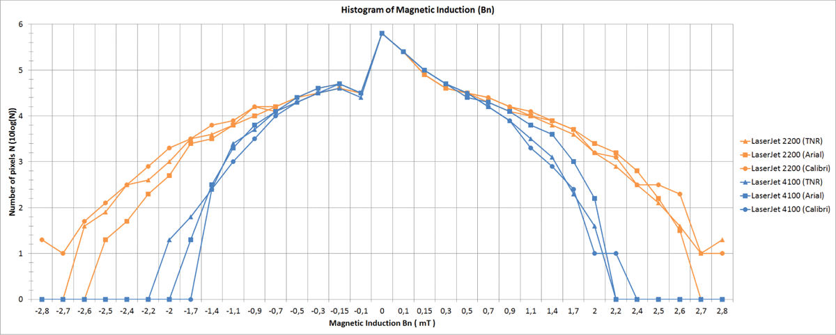
Figure C-1.
Six measurements of magnetic induction on two samples. On each sample the word “Bob” is measured on three different fonts.
This appendix shows the details of the calculation of the scores as displayed in Figure 9. On each sample three measurement are performed on the word “Bob”: once on the font Times New Roman (12pt), once on the font Arial (11pt) and once on the font Calibri (12pt).
This results in three columns (vectors) of data for each sample, as shown in Table C-1 and Figure C-1.
The 1-norm distance score (see Equation C-1) is calculated separately for each corresponding font. In other words, the measurement on the word “Bob” in the font Times New Roman (TNR) is compared to the word “Bob” in the font TNR on a different sample and likewise for the other two fonts.
As a final result, the three distance scores of the three fonts are averaged as the final 1-norm distance score between the two samples. If the two samples originate from the same printer, the score is labeled as “within variation” score. If the two samples originated from different printers, the score is labeled as “between variation” score.
The 1-norm distance score (P1) between two samples x and y with two columns (vectors) of n datapoints (xi and yi) is defined as:
C-1
[TeX:] \documentclass[10pt]{article} \usepackage{wasysym} \usepackage[substack]{amsmath} \usepackage{amsfonts} \usepackage{amssymb} \usepackage{amsbsy} \usepackage[mathscr]{eucal} \usepackage{mathrsfs} \usepackage{pmc} \usepackage[Euler]{upgreek} \pagestyle{empty} \oddsidemargin -1.0in \begin{document} \[ p^{1} = \sum_{i=1}^{n} \vert x_{i}- y_{i}\vert \] \end{document}And the total 1-norm distance score (P1total) is the average of the three distance scores calculated for the three different fonts.
C-2
[TeX:] \documentclass[10pt]{article} \usepackage{wasysym} \usepackage[substack]{amsmath} \usepackage{amsfonts} \usepackage{amssymb} \usepackage{amsbsy} \usepackage[mathscr]{eucal} \usepackage{mathrsfs} \usepackage{pmc} \usepackage[Euler]{upgreek} \pagestyle{empty} \oddsidemargin -1.0in \begin{document} \[ P^{1}_{total} = \frac{P_{TNR}^{1}+P_{Arial}^{1}+P_{Calibri}^{1}} {3} \] \end{document}In Table C-1 the calculation of the 1-norm distance score is shown for the font Times New Roman and the total 1-norm distance score is given below Table C-1.
Table C-1.
Measurement data (magnetic induction) and calculated distance scores for two samples (LaserJet 2200 and LaserJet 4100) and three fonts (Times New Roman, Arial and Calibri)
| Induction | LJ 2200 (TNR) | LJ 2200 (Arial) | LJ 2200 (Calibri) | LJ 4100 (TNR) | LJ 4100 (Arial) | LJ 4100 (Calibri) | | xi - yi | (TNR) | | xi - yi | (Arial) | | xi - yi | (Calibri) |
|---|---|---|---|---|---|---|---|---|---|
| -2.8 | 0 | 0 | 1.3 | 0 | 0 | 0 | 0 | 0 | 1,3 |
| -2.7 | 0 | 0 | 1 | 0 | 0 | 0 | 0 | 0 | 1 |
| -2.6 | 1.6 | 0 | 1.7 | 0 | 0 | 0 | 1,6 | 0 | 1,7 |
| -2.5 | 1.9 | 1.3 | 2.1 | 0 | 0 | 0 | 1,9 | 1,3 | 2,1 |
| -2.4 | 2.5 | 1.7 | 2.5 | 0 | 0 | 0 | 2,5 | 1,7 | 2,5 |
| -2.2 | 2.6 | 2.3 | 2.9 | 0 | 0 | 0 | 2,6 | 2,3 | 2,9 |
| -2 | 3 | 2.7 | 3.3 | 1.3 | 0 | 0 | 1,7 | 2,7 | 3,3 |
| -1.7 | 3.5 | 3.4 | 3.5 | 1.8 | 1.3 | 0 | 1,7 | 2,1 | 3,5 |
| -1.4 | 3.6 | 3.5 | 3.8 | 2.4 | 2.5 | 2.4 | 1,2 | 1 | 1,4 |
| -1.1 | 3.8 | 3.8 | 3.9 | 3.4 | 3.3 | 3 | 0,4 | 0,5 | 0,9 |
| -0.9 | 4.2 | 4 | 4.2 | 3.7 | 3.8 | 3.5 | 0,5 | 0,2 | 0,7 |
| -0.7 | 4.1 | 4.2 | 4.2 | 4.1 | 4.1 | 4 | 0 | 0,1 | 0,2 |
| -0.5 | 4.3 | 4.4 | 4.4 | 4.3 | 4.4 | 4.3 | 0 | 0 | 0,1 |
| -0.3 | 4.5 | 4.6 | 4.5 | 4.5 | 4.6 | 4.5 | 0 | 0 | 0 |
| -0.15 | 4.6 | 4.7 | 4.6 | 4.6 | 4.7 | 4.7 | 0 | 0 | 0,1 |
| -0.1 | 4.5 | 4.5 | 4.5 | 4.4 | 4.5 | 4.5 | 0,1 | 0 | 0 |
| 0 | 5.8 | 5.8 | 5.8 | 5.8 | 5.8 | 5.8 | 0 | 0 | 0 |
| 0.1 | 5.4 | 5.4 | 5.4 | 5.4 | 5.4 | 5.4 | 0 | 0 | 0 |
| 0.15 | 4.9 | 4.9 | 4.9 | 5 | 5 | 5 | 0,1 | 0,1 | 0,1 |
| 0.3 | 4.6 | 4.6 | 4.6 | 4.7 | 4.7 | 4.7 | 0,1 | 0,1 | 0,1 |
| 0.5 | 4.5 | 4.5 | 4.5 | 4.5 | 4.4 | 4.5 | 0 | 0,1 | 0 |
| 0.7 | 4.4 | 4.3 | 4.4 | 4.2 | 4.3 | 4.2 | 0,2 | 0 | 0,2 |
| 0.9 | 4.2 | 4.1 | 4.2 | 3.9 | 4.1 | 3.9 | 0,3 | 0 | 0,3 |
| 1.1 | 4 | 4 | 4.1 | 3.5 | 3.8 | 3.3 | 0,5 | 0,2 | 0,8 |
| 1.4 | 3.8 | 3.9 | 3.9 | 3.1 | 3.6 | 2.9 | 0,7 | 0,3 | 1 |
| 1.7 | 3.6 | 3.7 | 3.7 | 2.3 | 3 | 2.4 | 1,3 | 0,7 | 1,3 |
| 2 | 3.2 | 3.4 | 3.2 | 1.6 | 2.2 | 1 | 1,6 | 1,2 | 2,2 |
| 2.2 | 2.9 | 3.2 | 3.1 | 0 | 0 | 1 | 2,9 | 3,2 | 2,1 |
| 2.4 | 2.5 | 2.8 | 2.5 | 0 | 0 | 0 | 2,5 | 2,8 | 2,5 |
| 2.5 | 2.1 | 2.2 | 2.5 | 0 | 0 | 0 | 2,1 | 2,2 | 2,5 |
| 2.6 | 1.6 | 1.5 | 2.3 | 0 | 0 | 0 | 1,6 | 1,5 | 2,3 |
| 2.7 | 1 | 0 | 1 | 0 | 0 | 0 | 1 | 0 | 1 |
| 2.8 | 1.3 | 0 | 1 | 0 | 0 | 0 | 1,3 | 0 | 1 |
| P1 = ∑ = | 30,4 | 24,3 | 39,1 |
Notes
[2] Bn is the component of magnetic induction normal to the surface and not the total magnetic induction vector. However for the readability of this article, Bn will be simply called magnetic induction for the remainder of this article.
Acknowledgements
Special thanks go to Regula Forensics and Joost Vlek from Advanced Security Solutions BV for making the Regula Magmouse Model 4197 available to the Netherlands Forensic Institute for the measurements. Apart from lending the Magmouse, Regula was not involved in this study. Furthermore, most of the work of this study is done by Miriam Mieremet during her internship. Her report with more details can be found online at the repository of Delft University of Technology [6].