
1.0 Motivation
Hydrogen is believed to become an important future energy carrier aiming at the reduction of carbon dioxide emissions. Predicting flammability limits (FLs) for hydrogen mixtures as precisely as possible is an important piece of information for improving the safety of hydrogen applications. FLs are experimentally obtained using standardized procedures: the most common ones are ISO 10156 (Standardization, 2017)/DIN EN 1839 (Standardisation, 2017). There is an influence of initial temperature and pressure, and diluents, affecting the FLs (Hattwig and Steen, 2008). Limited, partly unevenly distributed experimental data exists. Most FLs experiments of hydrogen mixtures are conducted in air with inert gas admixtures such as nitrogen, argon, helium, steam, carbon dioxide, or a combination of these inert gases at ambient pressure. Some experimental data is available for hydrogen–oxygen mixtures. Thus, using this data for improving mathematical models becomes a challenge.
There are empirical models correlating FLs to temperature, indicating an increase in upper flammability limit (UFL) and a decrease in lower flammability limit (LFL) with an increase in initial temperature. These empirical linear equations are used (Ale, 1998; Arnaldos, Casal and Planas-Cuchi, 2001; Liaw and Chen, 2016; Mendiburu, Carvalho and Ju, 2023; Molnarne, Schendler and Schröder, 2008) to estimate the FLs at reduced pressure as a function of initial temperature. Equation 1 indicates this correlation:
For LL,U (mol %) being the LFL or UFL at temperature (T (K)). Lo (mol %) is the UFL or LFL in air at reference temperature (To), and K is an empirical correlation factor. This equation was initially established for determining the temperature-dependent LFLs of hydrocarbons. It is, however, noted in some literature (Qi et al., 2022) to indicate higher deviations on UFL predictions at high initial temperatures. Modifications to equation 1 were established (Kumar, 1985) to estimate the FLs in dependance from inert gas admixtures. For hydrogen–air–inert mixtures, an empirical model for determining UFLs and LFLs is reported in literature (Bade, 1993; Terpstra, 2012), relating the diluted mixtures to the undiluted fuel mixtures FLs using an experimentally obtained or calculated correlation factor. This empirical model indicates a reduction in accuracy for inert gas-rich mixtures, except for mixtures diluted with nitrogen.
The model of constant adiabatic flame temperature (CAFT) has also been often used in recent literature, in addition to the model of constant laminar flame velocity. The CAFT model implies that if the mixture calculated adiabatic flame temperature is above the reference flame temperature, the mixture is deemed flammable (Henriksen and Bjerketvedt, 2025; Dwyer, Hansel and Philips, 2003). This approach has been mainly used to estimate FLs of hydrocarbon fuel mixtures with good accuracy (Gasse, 1992; Mashuga and Crowl, 1999). However, deviations are observed when using this type of model by predicting mixtures with high inert diluent concentrations (Henriksen and Bjerketvedt, 2025). Moreover, the reference flame temperature is different for UFLs and LFLs. Modifications to the CAFT model have already been developed (Abdelkhalik et al., 2021). Gasse (Gasse, 1992) has incorporated the influence of Lewis numbers (Le) in the FL predictions, developing modified equations:
For ϑF,U, ϑA representing the flame temperature and initial temperature, respectively. The variable represents the inert gas composition. The fuel, air, and inert gas molar heat capacities are represented by , and . The variables vB and v02 represent the fuel and oxidizer stoichiometric coefficients. is the reaction enthalpy. This model considered the influence of temperatures, Lewis numbers, and mixture composition to determine the FLs.
Machine learning (ML) models have been used to predict LFLs and UFLs of hydrocarbons in air based on chemical and physical properties of the substances, applying a so-called quantitative structure–property relationship (QSPR) approach (Jiao et al., 2020; Pan et al., 2009; Yuan et al., 2019) to address the limitations of common empirical models. An effective ML modeling methodology has been implemented (Li, Liang and Han, 2024) to develop and analyze the performance of different ML classification algorithms, including the Decision Tree, Feedforward Neural Network, Support Vector as well as Random Forest models, to predict the conditions at which stoichiometric H2–O2 mixtures ignite spontaneously with respect to initial pressure dependence. Implementation of ML algorithms presents an opportunity to consider the influence of temperature and of admixtures of different types of inert gas on FLs. This can also include considering new types of inert gases by substituting them by reference inert gas mixtures with similar physical properties. Through literature revisions on FL determination and empirical modeling, the combined parameters, adiabatic flame temperature, initial pressure and temperature, mixture composition, and Lewis numbers, are crucial parameters for predicting FLs of the mixture.
Aiming at the development of an accurate and comprehensive model to predict the FLs of hydrogen, in dependence from temperature and admixtures of inert diluents, it is therefore an objective of this study to develop a multilayer perceptron (MLP) model at ambient pressure and varying initial temperature, incorporating additional feature input structures as well as implementing the models with the hyperparameter optimization algorithm. Input feature impacts on model performances were investigated, and the models were deployed for prediction analysis, whose results are evaluated against existing empirical flammability prediction models.
2.0 Methodology
2.1. Experimental data set and data augmentation
The study uses datasets from the CHEMSAFE database (at 1 bar) (CHEMSAFE, 2019; Molnarne, Schendler and Schröder, 2008), experimentally obtained according to DIN 51649-1 and DIN EN 1839 (Standardisation, 2017) for H2–Air mixtures diluted with Ar, CO2, N2, H2O, and He, at 293 K, 373 K, 473 K, 573 K, 673 K. A total of 350 datasets (i.e., experimentally determined FLs) were obtained, whose distribution per inert diluents is shown in Figure 1.
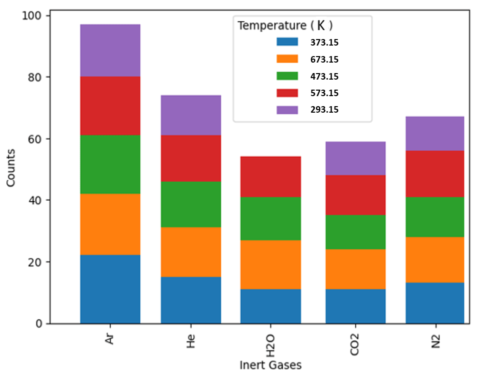
Figure 1
Flammability limits experimental data volume distribution (Molnarne, Schendler and Schröder, 2008).
According to the standards applied, the measurement uncertainties of the data are defined to be lower than ±0.2 mol% of hydrogen (Molnarne, Schendler and Schröder, 2008). Figure 2 depicts the influence of different inert gas admixtures on the explosion regions at 473K. This dependency is similar to all other initial temperatures considered in this study. Mixtures diluted with steam and carbon dioxide indicate relatively smaller explosion regions in comparison to those diluted with Ar, N2, or He. The mass and thermal diffusivity as well as the heat capacities of the mixtures differ and play a crucial role in the mixture’s FLs. Hence, this study seeks to utilize the MLP ML models to investigate the combined influence of these parameters and their effects on FLs prediction accuracies.
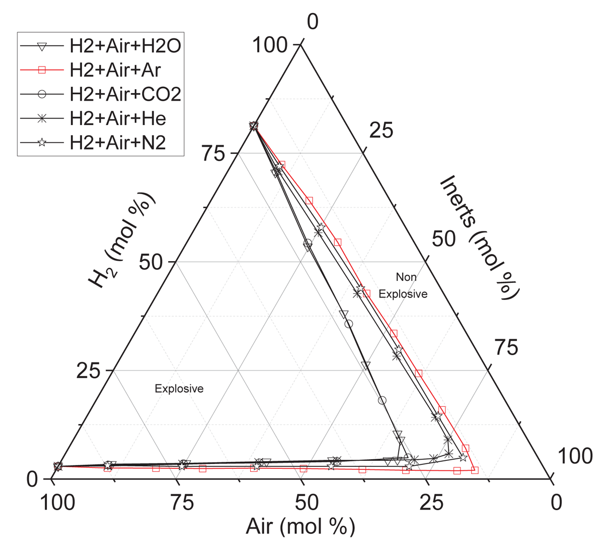
Figure 2
Influence of inert gas admixtures on explosion region (473.15 K) (Data from Molnarne, Schendler and Schröder, 2008).
For each flammability diagram at each temperature, a spline linear interpolation (Erdogan, 2013) was implemented on the experimental data. This established a series of mixtures (in steps of 1 mol % of inert gas) forming a continuous flammability classification boundary. Additional gas mixtures were defined by creating 10 layers inside (explosive – (1)) and 10 layers outside (non-explosive – (0)) the explosive region spaced at 0.2 mol % H2 step sizes, as illustrated in Figure 3. In total, about 37,605 gas mixtures were defined from 350 experimental datapoints using this method and classified either as explosive or non-explosive. This method further assists the model to generalize the classification boundary of flammable gas mixtures in ternary hydrogen/inert gas/air mixtures at different temperatures. Cantera toolkit (Goodwin et al., 2018) was used to calculate the fuel Lewis and oxidizer Lewis numbers and adiabatic flame temperature, and appended to the other data frame parameters: temperature, pressure, gas mixture composition, and the target variables (label).
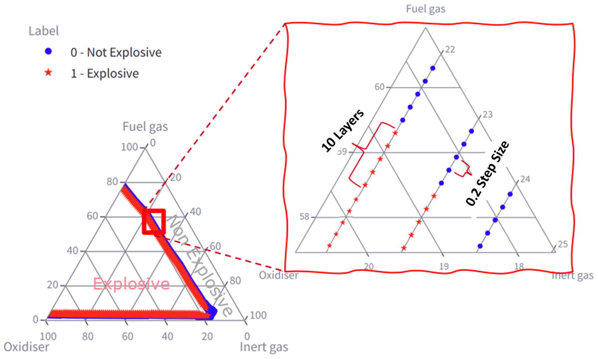
Figure 3
Data augmentation method (H2–Air–Ar data at 373.15 K).
2.2. Model input feature structures
To assess the influence of different features on the model performance, four different feature input structures were set up as indicated in Figure 4. They share similar physical implications with significant differences in how the mixture composition is presented to the MLP model structure.
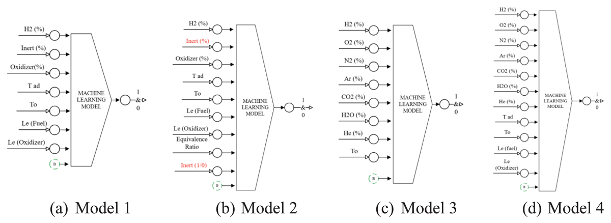
Figure 4
Models input feature structures.
To is the initial temperature and Tad is the calculated adiabatic flame temperature. Inert gas (1/0) in model 2 represents the one-hot-encoded state of specific inert gas type existence, whose gas fraction is provided by inert gas molar fraction in the gas mixture. B is the error term. Model 1 is focused on thermophysical characteristics of the mixtures as input parameters for the classification. The type of inert gas is not used as input feature directly, but only the inert gas fractions, assuming that the type of inert gas is reflected by its influence on the Tad and Lewis numbers (Le (fuel) and Le (oxidizer)). In model 2, the type of inert gas is directly fed by one-hot-encoding. In models 3 and 4, the type of inert gas is directly fed as single inert gas fraction. Model 3 serves as the control model, only using the mixture composition and initial temperature as input features without other computed thermophysical or thermodynamic properties. Due to the limitations of experimental data wherein inert diluted hydrogen mixtures were oxidized by pure oxygen, this study has only utilized air mixtures with air as oxidizer for training. In models 3 and 4, air as the oxidizer was separated into its components: oxygen, nitrogen, and argon, whereby Ar and N2 fractions were appended to their respective inerts fraction. Model 2 can determine the FLs of hydrogen–air mixtures at any temperature and with any type of inert gas, but is limited to mixtures with single inert gas dilution. Models 1, 3, and 4 can predict FLs for mixtures with combined inert gases.
A two-level factor Taguchi L16 orthogonal array (Kaur et al., 2023; Lazić, 2013; Munger and Desa, 2021) was used to investigate the main effects of five neural network hyperparameters, as indicated in Table 1, while ensuring a balanced factor combination.
Table 1
Process parameters and variables.
| FACTORS | LEVEL 1 | LEVEL 2 |
|---|---|---|
| A. Hidden Layers | • 120,60,30 | • 100,50 |
| B. Solver | • lbfgs | • Adam |
| C. Alpha | •0.00001 | • 0.001 |
| D. Activation Function | • tanh | • ReLU |
| E. Learning Rate | • constant | • adaptive |
Furthermore, data were intentionally separated into five folds: each fold represents a specific temperature (293 K, 373 K, 473 K, 573 K, and 673 K), and a five-fold cross-validation process was implemented on the model during training and validation. This implies that the model holds one-fold as testing data and uses the remaining four folds for training, further enabling the hyperparameter optimization process implementation: the model trains and validates with each hyperparameter set from the hyperparameter pool. All models were trained with 1000 iterations and a 42 random state. The best hyperparameters obtained for models are indicated in Table 2.
Table 2
Optimized model hyperparameters.
| HYPERPARAMETERS | MODEL 1 | MODEL 2 | MODEL 3 | MODEL 4 |
|---|---|---|---|---|
| Hidden layer structure | 120,60,30 | 120,60,30 | 120,60,30 | 120,60,30 |
| Activation function | ReLU | ReLU | tanh | tanh |
| Solver function | adam | lbfgs | adam | adam |
| Alpha | 0,001 | 0,001 | 0,00001 | 0,00001 |
| Learning rate | constant | constant | adaptive | adaptive |
The model’s validation and testing approach, adapted herein, was similarly based on experimental flammability determination process: (a) H2 concentration was varied in discrete steps (0.2 mol % H2) at fixed inert gas fractions and initial temperature, (b) the flammability state (Labels) of the gas was observed until the boundary between explosive and non-explosive mixtures was found. The apex accuracy was tested by systematically increasing the inert mole fraction in discrete step sizes until the UFL and LFL merge. The accuracy evaluation metrics used herein are based on the absolute deviations between the predicted and corresponding test FLs at similar initial conditions: absolute deviations for the UFL, LFL (mol % H2), and apex (mol % inert gas).
2.3. Feature impacts on model prediction analysis
The relative impacts of the individual features on the model’s prediction performances were analyzed using the Shapley Additive exPlanations (SHAP) values (Antonini et al., 2024; Lubo-Robles et al., 2020; Marcílio and Eler, 2020) wherein the SHAP values are being used to interpret ML model predictions with respect to the input variables. Figure 5 exemplary depicts the feature impacts (for 500 well-distributed samples) on model 4 predictions. The colors represent the positive or negative correlation of a feature, while SHAP values on the x-axis imply the probability of the predicted mixtures being flammable or non-flammable.
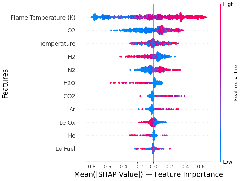
Figure 5
Model 4 mean SHAP values summary plot.
A physical implication of the individual features on FLs is clearly observable in Figure 5. The mixture adiabatic flame temperature has the highest impact of all features on the model prediction, with a wider spread on the SHAP values. As expected, lower flame temperature and oxidizer content (oxygen/air) tend to decrease the probability of flammability. The influence of the fuel Lewis number seems to have the least impact on the prediction, with ambiguous tendency. The Lewis oxidizer is also noted to have the least narrow impact on the model prediction. However, their inclusion in training and testing can have benefits in assisting the models in capturing the heat and mass transfer effects of various gas mixtures on FLs. Both models 1 and 2 were similarly largely influenced by the adiabatic flame temperature and initial temperature, with model 2 also equally largely impacted by the equivalence ratio. Overall, an optimum combination of these features is beneficial for the model prediction due to their different effects on the model performance at all levels of feature values.
3.0 Results
3.1. Model validation
The model’s performance during testing was evaluated by the mean deviations of predicted UFLs and LFLs with respect to the test datasets. Deviations at the apex were also captured. Exemplarily, Figure 6 depicts the models’ performances on the best chosen hyperparameters at different temperature validation folds (averaged across inert gas diluents).
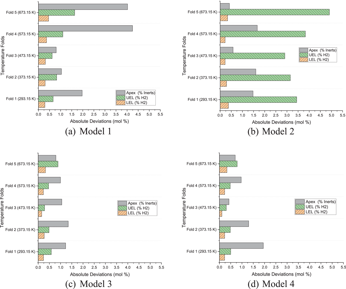
Figure 6
Model’s best hyperparameter performances on models cross-fold validation.
Due to the nature of model validation implemented, the influence of extrapolation is observable on the models’ performance on temperature folds 1 and 5. Model 1 indicated high apex absolute mean deviations among these models. Models 3 and 4 performances on validation data temperature folds 2, 3, and 4 indicate similar deviations comparable to the UFL and LFL experimental determination tolerance. Model 4 indicates high apex deviations at temperature fold 1 in comparison to model 3. In comparison to model 1, model 2 has, however, indicated improved performance on apex determination, but the highest UFL average deviations among all models. The overall performance for all models’ prediction on UFL, LFL, and apex performance, averaged across inert gas admixtures and initial temperature, is depicted in Figure 7.
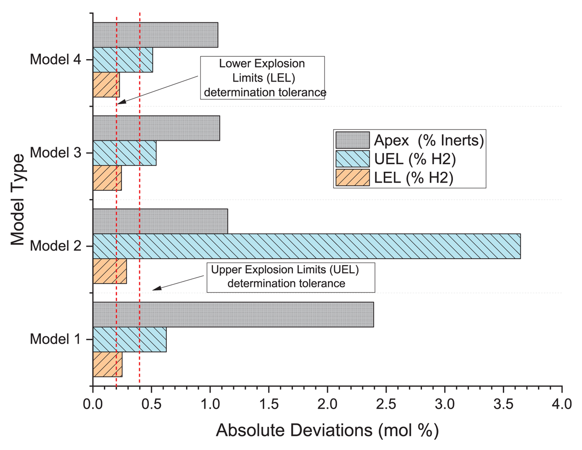
Figure 7
Overall model’s prediction.
On average, models 3 and 4’s prediction performances on testing data are better in comparison to models 1 and 2. The average deviations of LFLs and UFLs of models 3 and 4 from the test values are comparable to the levels of experimental flammability determination tolerance given for gases with similar FLs: LFL (±0.2% H2) and UFL (±0.4% H2) (Standardisation, 2017). For the apex, no experimental determination tolerance is given in the standard, but considering the more complex experimental determination procedure and the step size for variation of inert gas fraction of 0.5 mol %, it can be expected that it is significantly larger than for LFL and UFL determination. Across the model types, the differences in performance were not significant between models 3 and 4. Due to the poor performance of model 1 and limitations on model 2 (only applicable to predicting mixtures with single inert gases), only models 3 and 4 are subjected to further testing on extrapolation to O2 oxidized mixtures, as well as mixtures with multiple inert gas admixtures. Some mixtures at certain temperatures indicate high deviations at high inert gas fractions and for the apex, affecting the averaged absolute deviations, as observable in Figures 8 and 9. Exemplarily, Figure 8 shows the LFL prediction performances of models 3 and 4 on various inert gas admixtures.
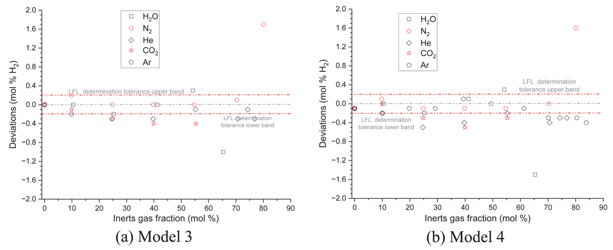
Figure 8
Models 3 and 4 LFL prediction deviations (473.15 K).
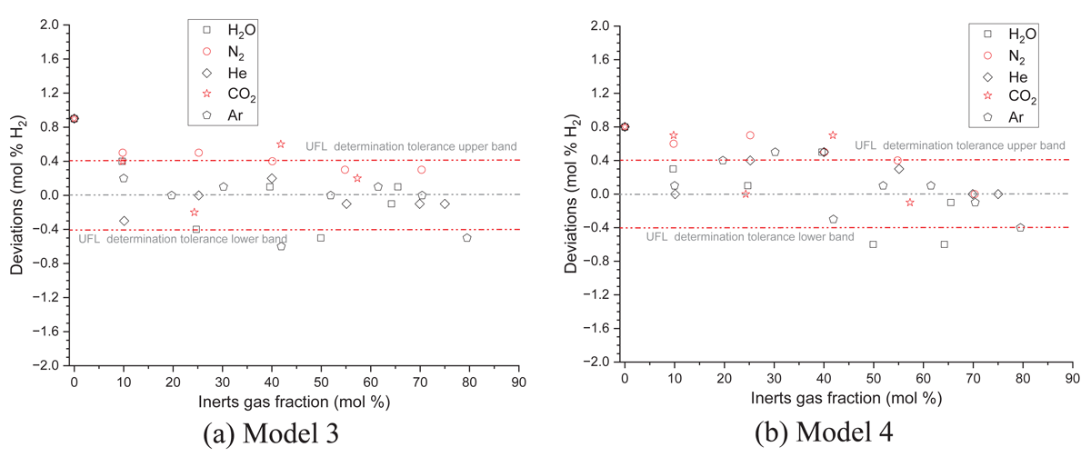
Figure 9
Models 3 and 4 UFL prediction deviations (473.15 K).
For fuel-rich mixtures, models 3 and 4 LFL prediction deviations are well within or near the ±0.2 mol % H2 tolerance. At higher inert gas dilutions, deviations of predicted LFL from experimental values are significant, especially for model 3 and model 4 predictions on H2O and N2 diluted mixtures. Models 3 and 4 have also indicated good performance in predicting UFL of diluted H2/air mixtures as depicted in Figure 9. The distribution of most computed deviations falls within the experimental tolerance band (±0.4 mol % H2). Both models 3 and 4 have underpredicted the undiluted mixtures UFLs by 0.8% H2.
Mixtures at UFL are fuel-rich, i.e., Φ > 1. Thus, for the UFL, air is the limiting factor, hence an absolute deviation of 0.5 mol% H2 in air approximately corresponds to a change of about only 0.1 mol% of the actual oxidizing species oxygen. This implies that the accuracy of UFLs predictions is comparable to the accuracy of the prediction of the LFLs. The distribution of the absolute mean deviations between models 3 and 4 could also highlight the influence of additional parameters: fuel and oxidizer Lewis numbers and adiabatic flame temperature.
Model comparison to empirical model
Models 3 and 4 performances were further evaluated by comparing their prediction performances against predictions from simple empirical linear models for predicting the FLs in dependence from initial temperature (equation 1), as indicated in Figure 10. The empirical linear models’ correlation factors (KLFL and KUFL) were empirically determined by fixing To and T at 293 K and 673 K, respectively, using their referenced undiluted mixtures LFL and UFL.
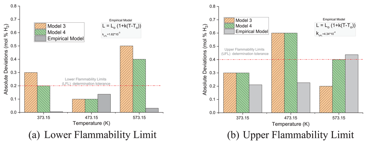
Figure 10
ML performances on FL temperature dependency compared to simpler linear empirical model (equation 1).
For the UFLs, at 373.15 K, both the MLP models indicate comparable absolute deviation, while the empirical model shows a lower deviation of about 0.2 mol % H2, well below the UFL experimental determination tolerance. At 473.15 K, prediction deviations for the MLP models are above the UFL experimental determination tolerance by 0.1% H2, while the empirical model prediction absolute deviation remains constant. At 573.15 K, model 3 indicates the lowest prediction deviation among the three models, while the empirical model and model 4 indicate higher deviations of about 0.44% H2 and 0.4% H2, respectively. This indicates that the empirical model performs more consistently across these temperatures, while the MLP models indicate temperature-dependent behavior (notable at 473.15 K). Overall, the UFL prediction deviations are comparable to the experimental UFL determination tolerance. The noted high prediction deviations at 473.15 K could be due to shortcomings of the MLP ML models: the MLP model interpolates non-globally using multiple local nonlinear regions. For the LFL predictions, however, the MLP models indicated higher prediction deviations at 573.15 K; model 3 predicts with 0.5% H2 deviations, while model 4 is 0.1% H2 deviations less than model 3. However, at 473.15 K, the prediction deviations of both MLP models are lower than that of the empirical model. The ML models’ performance is comparable, especially on the UFL predictions, where the empirical models are known to be less accurate in predicting FLs for hydrocarbons or hydrogen mixtures. When comparing the models, the very different application ranges of the models must be taken into account. The empirical model is limited to the temperature dependency of undiluted hydrogen–air mixtures.
Similarly, the models were also validated against the semi-empirical models of CAFT discussed in equations 2 and 3, on their ability to determine the maximum inert gas molar concentration required (apex) for mixtures to be explosive. An overview of the ML models (models 3 and 4) performance on apex determination in comparison to the semi-empirical calculations by Gasse (1992) is shown in Table 3.
Table 3
Apex determination evaluation (473.15 K).
| INERT GAS ADMIXTURES (MOL % INERTS) | |||||
|---|---|---|---|---|---|
| CO2 | H2O | HE | N2 | AR | |
| Experimental Data | 69.6 | 68.1 | 78.1 | 84.0 | 84.5 |
| MODEL PREDICTIONS ABSOLUTE DEVIATIONS (MOL % INERTS) | |||||
| Gasse model (eqs. 2 and 3) | 11.0 | 19.4 | 5.2 | 0.2 | 3.9 |
| Model 3 | 0.6 | 1.2 | 1.3 | 3.4 | 0.4 |
| Model 4 | 0.8 | 1.25 | 0.9 | 3.0 | 0.1 |
The semi-empirical CAFT model strongly overpredicts the apex for H2/Air mixtures diluted with CO2, H2O, He, and Ar. The ML models tend to improve the apex determination accuracy: reduction in apex prediction inaccuracies on CO2, H2O, He, and Ar diluted mixtures. Nevertheless, the ML model performances on N2-diluted mixtures tend to overpredict the apex stronger by 3.0% N2 in comparison to the CAFT model predictions. This further illustrates that the current ML model could have benefits when predicting the apex in comparison to the CAFT semi-empirical model. As ML models are flexible, additional parameters can be introduced to further improve these models’ prediction performances.
3.2. Model extrapolation to H2/O2/N2 mixtures and mixtures with multiple inert gases
Consideration of air separation into its primary components enables models 3 and 4 to extrapolate onto the H2–O2–inert explosion region and determine the FLs for these kinds of mixtures. In Figure 11, the results of models 3 and 4 extrapolations on these explosion regions are depicted. For mixtures with a ratio of oxygen to nitrogen equivalent to or lower than that in air (H2–air–N2 mixtures) (gray region in Figure 11, equaling the ternary system of H2–air–N2), it can be observed that both models 3 and 4 make predictions of FLs with good accuracies comparable to the models’ test performances when using air as the oxidizer. Model 4 has generally indicated good extrapolation on the LFLs of gas mixtures outside the air-oxidized gas mixture ranges. It only starts to fail at very low nitrogen fractions below 5 mol%. Model 3 predictions have significant absolute deviations up to 4% H2 on the LFL for non-diluted H2–O2 mixtures.
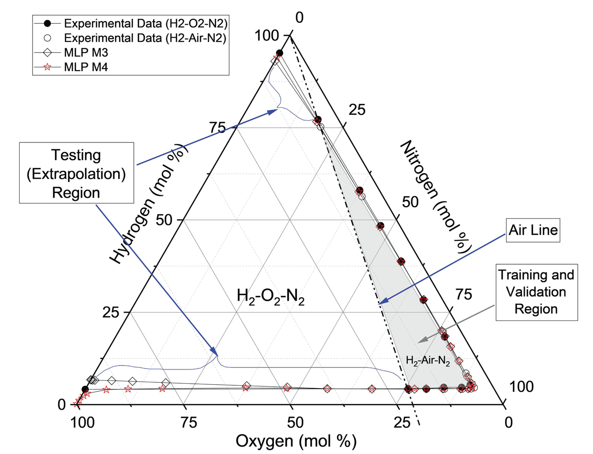
Figure 11
Models extrapolation to H2–O2–N2 gas mixtures (293.15 K).
For H2-O2 mixtures without N2, both models underpredicted the UFL with deviations; model 3 (2.2 mol % H2) and model 4 (1.2 mol % H2), from the experimental data. Higher prediction deviations for undiluted mixtures are mainly due to the lack of experimental data on these regions, as the model has never generalized these explosion regions. Nevertheless, in extrapolating FLs to H2–O2–N2 mixtures, model 4 indicates a better performance than model 3. Model 4 performance, especially at LFL of undiluted mixtures, could further be improved by introducing more training parameters, which are not covered in the scope of this study.
These two models were further validated by extrapolating to mixtures consisting of multiple inert gas admixtures: the models were trained using mixtures with single inert gas admixtures. This is mainly due to the limited volume and distribution of experimental data of these types of gas mixtures. The performance of models 3 and 4 on these kinds of mixtures is as depicted in Figure 12. The experimental data used to validate these models’ predictions on inert gas interpolations were obtained from Gasse (1992).
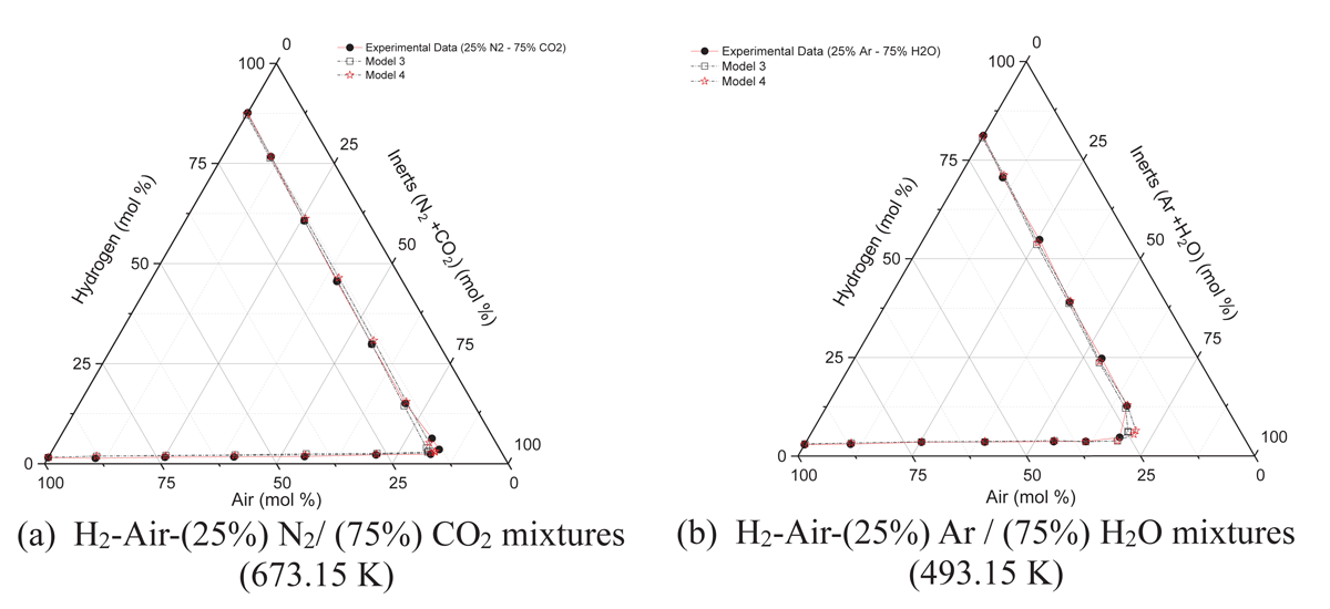
Figure 12
Models’ extrapolation on mixtures with multiple inert gases.
Both models indicated good performances in determining the FLs on both mixtures. These models’ average absolute deviations are indicated in Table 4.
Table 4
Summary of models’ absolute deviations of extrapolation of multiple inert gases diluted H2-air mixtures.
| MIXTURES | ||||
|---|---|---|---|---|
| H2–Air–(25%) N2/(75%) CO2 (673.15 K) | H2–Air–(25%) Ar/(75%) H2O (493.15 K) | |||
| MODELS ABSOLUTE DEVIATIONS | ||||
| MODEL 3 | MODEL 4 | MODEL 3 | MODEL 4 | |
| LFL (mol % H2) | 0.45 | 0.33 | 0.27 | 0.27 |
| UFL (mol % H2) | 0.58 | 0.59 | 0.67 | 0.47 |
| Apex (mol % Inerts) | 2.16 | 0.65 | None | None |
Overall, model 4 performed slightly better than model 3 in predicting both UFLs and LFLs for the tested mixtures. This is further illustrated on apex determination accuracy on N2/CO2 diluted mixtures, with model 4 indicating a much lower apex deviation. For the Ar/H2O diluted mixtures, there was no experimental data provided for the apex. Both models’ prediction absolute deviations are just slightly above the required LFL and UFL experimental tolerances. More parameters can be introduced into the models to further assess their performance by predicting mixtures consisting of different proportions of different inert gases.
4.0 Conclusion and Recommendations
In this study, FLs for hydrogen mixtures are comprehensively predicted for initial temperature and inert gas admixtures with improved accuracy using an optimized MLP model. Four different models defined by four different key input feature sets composed of mixture composition (distinctive mixture elements), initial temperature, Lewis numbers, and adiabatic flame temperature were used. A total of 350 experimentally determined FLs were extracted from the CHEMSAFE database and augmented to define 37,605 gas mixtures classified as explosive or non-explosive. Cantera was implemented to compute thermophysical parameters and flame temperatures. Hyperparameter optimization was implemented to assist in selecting the model parameters with the least averaged deviations on LFL, UFL, and apex. The models were evaluated using a temperature hold-out method: systematically holding out all data at a specific temperature, hence used for model testing (while training the models using the remaining datasets).
Models 3 and 4, which use all inert gas fractions directly as input features, indicated least average deviations. Overall, models 3 and 4 delivered least absolute mean deviations (averaged across temperature and inert gases performance) on LFL (0.24 mol% H2 and 0.23 mol% H2, respectively), UFL (0.54 mol% H2 and 0.51 mol% H2, respectively), and averaged apex (both models at 1.1 mol% inerts). These absolute deviations are within the range of the respective LFL and UFL experimental FLs determination level of uncertainties. While model 3 uses only mixture composition and initial temperature as input parameters, model 4 is additionally fed with thermophysical parameters (Lefuel and LeOxidizer) and the adiabatic flame temperature (Tad), which are known to be relevant for the classification from other established models like the CAFT model. However, though especially the Tad is the input feature with the highest impact on the model 4 predictions, the model performance is not improved compared to model 3 overall, with exceptions on extrapolations. There are some indications for the benefits of thermophysical parameters incorporated in model 4 in case of extrapolations. On tested mixtures with multiple inert gas dilutions (H2/Air/CO2/N2 and H2/Air/Ar/H2O), models 3 and 4 also indicated averaged absolute deviations of LFL and UFL comparable to the respective LFL and UFL experimental FLs determination tolerances.
The models discussed herein are limited to hydrogen as fuel gas. It would be desirable to add fuel gases, especially NH3 and CH4, into the model, enabling computation of multiple fuel gas mixture limits of flammability. Further developments of the models to hydrocarbon fuel gas in the future works will show if a benefit in considering Tad for the prediction can be observed, as the CAFT model is known to be more accurate for hydrocarbon mixtures than for hydrogen mixture FLs determination. Both models 3 and 4 indicate good capability for extrapolation on mixtures outside their training boundaries (H2–O2–inerts) as well as on mixtures diluted with multiple inert gas admixtures. Also, both models deliver similar prediction accuracies comparable to the established empirical and semi-empirical models, while being more comprehensive with wider applicability and higher extrapolation potential. Future work on the models will feature further validation of the model performance, e.g., using different ML algorithms: support vector machines and random forests. This aims at further improving the models’ performance while improving the interpretability of the models. The current model will be made available upon request.
Competing Interests
The authors have no competing interests to declare.