
1.0 Introduction
The development and establishment of CO2-free drive systems is essential for driving forward the energy transition and reducing emissions in the mobility sector; this applies to both hydrogen and battery drives. Both drives are strongly linked to the infrastructure, with fast refueling and charging times being essential. However, fast hydrogen refueling leads to increased tank temperatures, impacting both fuel capacity and safety. This temperature rise results from the compression of hydrogen to high pressures during refueling. Since active cooling of the tank is impractical in mobile applications due to system complexity, space constraints, weight, and energy requirements, heat can only dissipate through convection to the environment or conduction to adjacent components.
The total heat generated depends on the refueled mass rather than the refueling time. However, with shorter refueling durations, less heat dissipates before completion, resulting in higher final tank temperatures. Elevated temperatures are undesirable for two main reasons. Firstly, higher temperatures lead to a lower hydrogen density at a given pressure, and consequently, the tank holds less hydrogen mass. In practice, as the tank cools after refueling, pressure drops below the target 350/700 bar. The state-of-charge (SOC) metric, as defined by SAE (SAE International, 2020), expresses the actual hydrogen density in the tank as a ratio relative to the density at nominal working pressure (NWP) and 15°C.
Secondly, excessive temperatures affect tank integrity, particularly for composite Type III and IV tanks commonly used in mobile applications. These tanks consist of an inner liner and an outer composite layer, which may separate at high temperatures, compromising structural integrity and increasing the risk of hydrogen leakage (Zhang et al., 2019). Industry guidelines, including those from SAE and manufacturers, set an 85°C temperature limit to prevent such risks (SAE International, 2020).
Several factors influence maximum tank temperature during refueling, including ambient conditions, initial tank pressure and temperature, pressure ramp rates, mass flow profiles, hydrogen inlet temperature, and tank design parameters such as material properties, volume, and geometry (Li et al., 2012; Gebhart et al., 2023; Klopčič et al., 2024; Bourgeois et al., 2018). Studies show that tank length-to-diameter ratios significantly affect temperature distribution and hot spot locations, making predictions challenging (Li et al., 2012). Tanks with low length-to-diameter ratios exhibit more uniform temperature fields, whereas larger tanks show strong temperature gradients (Gebhart et al., 2023; Klopčič et al., 2024; Martin et al., 2023; Kesana et al., 2023). According to Li et al. (2012), the location of these hot spots can change throughout the refueling process. Two primary phenomena contribute to the formation of hot spots: axial temperature gradients in larger tanks with high length-to-diameter ratios, where the hottest zone is often at the tank’s end (Kesana et al., 2023), and stratification, where vertical temperature gradients form due to buoyancy effects (Martin et al., 2023; Melideo et al., 2019; Gonin et al., 2023b).
For light-duty vehicles with tanks under 100 L, standardized refueling protocols exist under SAE J2601. These protocols utilize pre-cooled hydrogen (–40°C) and pressure ramp rates ranging from 5.1 to 28.5 MPa/min to achieve optimal SOC despite required overfilling (SAE International, 2020). In contrast, for heavy-duty refueling, the SAE J2601–5 guidelines were published in 2024, which provide refueling protocols for heavy-duty vehicles for the first time (SAE International, 2024). However, meeting refueling targets for heavy-duty applications, such as buses, trucks, and trains, still requires up to a 50% reduction in refueling times (Bölkov, 2023).
Hydrogen pre-cooling can mitigate temperature rise and reduce refueling duration, but optimizing this process requires balancing cooling energy demand. A comprehensive understanding of the refueling process is necessary, combining experimental studies and simulations. Experimental approaches involve thermocouples to identify temperature hot spots (Bourgeois et al., 2018; Martin et al., 2023), but these setups are challenging for large tanks and impractical for commercial applications. Even with tank-station communication for optimized refueling rates, built-in on-tank temperature sensors may not capture the actual peak temperature. Communicating a lower temperature could prompt the station to increase the filling speed, potentially having serious safety implications.
A further important aspect to consider when designing the tank system, especially for trucks, is packaging. The available packaging space limits possible tank sizes and geometries. To allow for more flexibility, vertical tank placement could be advantageous, but again leads to hot spots due to buoyancy effects.
Testing several tank geometries and filling conditions with elaborate measuring contraptions with spatially distributed temperature sensors is not feasible, especially for larger tanks. Therefore, simulation models are essential, broadly categorized into 0D thermodynamic models and 2D/3D computational fluid dynamics (CFD) models (Martin et al., 2023). The former enables rapid parametric studies, while the latter provides spatial temperature distributions and hot spot identification. Since each approach has strengths and limitations, integrating both experimental and simulation-based methods is necessary to advance refueling strategies. In this work, experimental as well as simulation results of three different tanks are presented to give further insight into the temperature distribution, hot spots, and safety-related challenges.
2.0 Methodology
In this chapter, the methodology employed will be presented. In total, three different tanks have been investigated: Type III 58 L tank (Tank A), Type III 320 L (Tank B), and Type IV 178 L (Tank C). Additional information on the three tanks is summarized in Table 1. Tank A and Tank B are shown in Figure 1. The former was integrated into a test rig of two identical tanks, but only one of the tanks was filled during the tests performed in this work. In addition to experimental investigations, 3D CFD simulations were conducted with Tanks A and C to calculate and observe the spatially resolved temperature field within the tank. The experimental and simulation methodology are presented in the subsequent sections.
Table 1
Investigated tank types and geometries.
| TANK | TANK TYPE | MAIN APPLICATION | VOLUME [L] | LENGTH [mm] | DIAMETER [mm] | PRESSURE [bar] |
|---|---|---|---|---|---|---|
| A | III | Car | 58 | 1100 | 324 | 700 |
| B | III | Bus | 320 | 3128 | 417 | 350 |
| C | IV | Heavy-duty | 178 | 1720 | 440 | 350 |
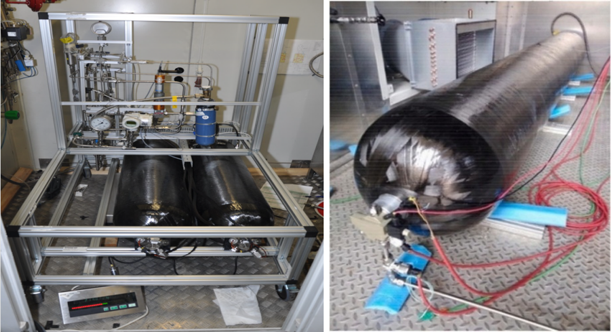
Figure 1
Tank A in test rig (left) and Tank B in test chamber (right).
2.1 Experimental setup
The experimental setup for all tanks tested within this work is similar, and is shown in Figure 2. Hydrogen from an 875 bar high-pressure storage is regulated via a pressure regulator valve to achieve the desired pressure ramp rate. A heat exchanger can be either bypassed or used for cold fill as low as –40°C. At this point, the hydrogen mass flow (MF1, Coriolis), temperature (TT1, PTC sensor inflow), and pressure (PT1) are measured. From there, hydrogen is supplied to the test chamber, where another temperature (TT2, thermocouple on pipe) and pressure (PT2) measurement occurs before the on-tank valve (OTV) at the tank inlet. Lastly, the OTV has an integrated temperature (TT3) and pressure (PT3) sensor to measure the thermodynamic states within the tank. For some tests, additional thermocouples were placed on the outer tank surface. In the case of Tank A, a measurement rod with five axially placed thermocouples was installed at the end-plug, thus the tank temperature could be measured at five locations within the tank. For Tanks B and C, no such measurement rod was available. Instead, the same type of OTV was installed at both tank ends, so that the inner tank temperature in front and at the back could be measured.
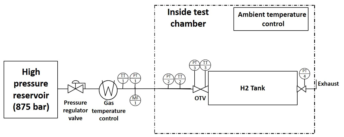
Figure 2
Scheme of test layout and sensors. Adapted from (Klopčič et al., 2024) according to CC-BY-4.0.
The test matrix for the different experiments is shown in Table 2. For the three test scenarios, Tank A was filled starting from 30 to 700 bar in approximately 6 minutes, which results in an APPR of 111.7 bar/min. The hydrogen was pre-cooled to –40°C in all cases. The ambient temperature was not regulated and was measured at around 6°C during the time of the tests. The main point of investigation with this tank was the impact of tank orientation on the temperature distribution in the tank. As seen in Figure 1, the test rig allows the tanks to be refueled either horizontally or vertically. The vertical case can further be divided in filling from below or from above depending on the orientation of the OTV.
Table 2
Test matrix.
| TEST Nr. | TANK | T AMBIENT [°C] | T H2 [°C] | p START [bar] | p TARGET [bar] | APPR [bar/min] | TANK ORIENTATION |
|---|---|---|---|---|---|---|---|
| 1 | A | 6 | –40 | 30 | 700 | 111.7 | vertical, filling from below |
| 2 | A | 6 | –40 | 30 | 700 | 111.7 | horizontal |
| 3 | A | 6 | –40 | 30 | 700 | 111.7 | vertical, filling from above |
| 4 | B | 15 | –40 | 30 | 350 | 50 | horizontal |
| 5 | B | 15 | –20 | 30 | 350 | 50 | horizontal |
| 6 | B | 15 | 0 | 30 | 350 | 50 | horizontal |
| 7 | B | 15 | –40 | 30 | 350 | 75 | horizontal |
| 8 | B | 15 | –20 | 30 | 350 | 75 | horizontal |
| 9 | B | 15 | 0 | 30 | 350 | 75 | horizontal |
| 10 | B | 15 | –40 | 30 | 350 | 100 | horizontal |
| 11 | B | 15 | –20 | 30 | 350 | 100 | horizontal |
| 12 | B | 15 | 0 | 30 | 350 | 100 | horizontal |
| 13 | C | 30 | 15–18 | 5 | 438 | 86.6 | horizontal |
| 14 | C | 30 | 15–18 | 5 | 438 | 43.3 | horizontal |
| 15 | C | 30 | 15–18 | 100 | 438 | 66.7 | horizontal |
The second investigated tank, Tank B, is for heavy-duty/bus applications and has a nominal working pressure of 350 bar. The main goal of the tests was to determine the effects of different refueling parameters on the final tank temperature. The two parameters that vary are the average pressure ramp rate (50, 75, and 100 bar/min) and cold-fill temperature (–40, –20, and 0°C), yielding a total of nine tests with all combinations of the two parameter values. The starting pressure in all cases was 30 bar, and the temperature of the climate chamber was regulated to 15°C. Due to restrictions in the testing time frame, it was not possible to design a custom contraption with spatially distributed thermocouples to measure the temperature field within the tank akin to Tank A. Thus, a second OTV was installed at the other tank end to at least measure the temperature at two positions.
Lastly, tests with Tank C were conducted to investigate the effect of filling time (5 or 10 min) and starting pressure (5 or 100 bar) on the tank temperature. The target pressure for the filling process was 438 bar (125% of nominal working pressure). The ambient temperature was controlled at 30°C and no pre-cooling of hydrogen was active. This resulted in hydrogen inflowing at 15–18°C, which was the ambient temperature at the high-pressure hydrogen supply. The relatively high ambient temperature and lack of pre-cooling were chosen specifically to represent a ‘worst case’ for the temperature of the Type IV tank. Analogous to Tank B, a second OTV with a temperature sensor was installed at the other tank end. Since it was expected that the temperatures may exceed 85°C, a termination condition was implemented to stop the filling process as soon as any of the two sensors displayed 85°C.
For comparison of experimental data with 0D as well as 3D CFD models, the average tank temperature is of interest. By employing an equation of state (e.g., Helmholtz free energy formulation in CoolProp (Bell et al., 2014)), the average tank temperature can be calculated based on the measured tank pressure and the hydrogen density in the tank. The latter can be obtained from the hydrogen mass in the tank (integral of the measured mass flow over time) and tank volume. The initial tank volume was known from the manufacturer, and a 1% volume increase at maximum pressure was estimated based on the measured change in circumference (axial expansion was neglected). For simplicity, a linear volume increase over the filling process was assumed.
2.2 Simulation
This section will present the 3D Computational Fluid Dynamics (CFD) model. The primary advantage of using a 3D CFD model over a 0D model lies in its ability to provide spatial resolution of the temperature field, eliminating the need for complex heat transfer correlations. As highlighted, the non-uniform temperature distribution within the tank during refueling leads to the presence of ‘hot spots’, which could pose a significant risk of material failure if temperatures locally exceed 85°C.
Despite its advantages, the 3D CFD model has significant limitations, mainly the high computational costs—calculating one refueling process can take over a month, depending on available computational infrastructure [115]. To reduce computational time, sacrifices in accuracy are made by using less computationally intensive turbulence and real gas models, or by simplifying the model to 2D axisymmetric versions (Bourgeois et al., 2018; Suryan, Kim and Setoguchi, 2013). Still, the 3D CFD models are not suitable for rapid design studies or parameter analyses. However, employing 3D CFD is essential for a deeper understanding of the refueling process under various conditions and for different tanks, as it provides insights into the spatial distribution of temperatures and the location of hot spots.
The geometry for the tanks was designed in the Computer Aided Design program SpaceClaim and includes both the fluid zone and the solid tank wall layers, including the valve. Five domains were considered in the simulation, as depicted in Figure 3: 1) Hydrogen in the tank, 2) Cold hydrogen in the nozzle filling the tank, 3) Aluminum valve, 4) Inner liner (Aluminum for Tank A, composite for Tank C), and 5) Outer layer from a composite material (carbon-fiber-reinforced polymer + epoxy resin).
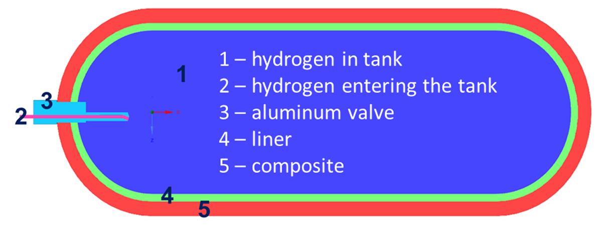
Figure 3
CAD model of the tank geometry with fluid and solid zones.
Using Ansys© Fluent’s meshing tool, a computational mesh was created with polyhedral elements, as exemplarily shown in Figure 4. To enhance solution accuracy, local refinement was applied in areas with high pressure gradients, particularly after the valve outlet where cold hydrogen enters the tank. A boundary layer of five layers was added at all fluid-solid interfaces to accurately model the turbulence near the walls. The nozzle area was extended slightly beyond the valve to allow the turbulent flow to fully develop before reaching the valve interface. A mesh independency study was conducted to determine the optimal cell count that maintains accuracy without significantly impacting the simulation results. Only the first five seconds of the refueling process were simulated to focus on the period of greatest temperature increase, as evidenced by the slope of the tank temperature profiles obtained experimentally. The total cell count of the final mesh for Tank A was approximately 300,000. For Tank C, the cell sizes were the same size as Tank A, but due to the higher volume, this resulted in a total cell count slightly above one million cells. The mesh remained stationary during simulation, thus not accounting for any volume expansion due to pressure build-up.
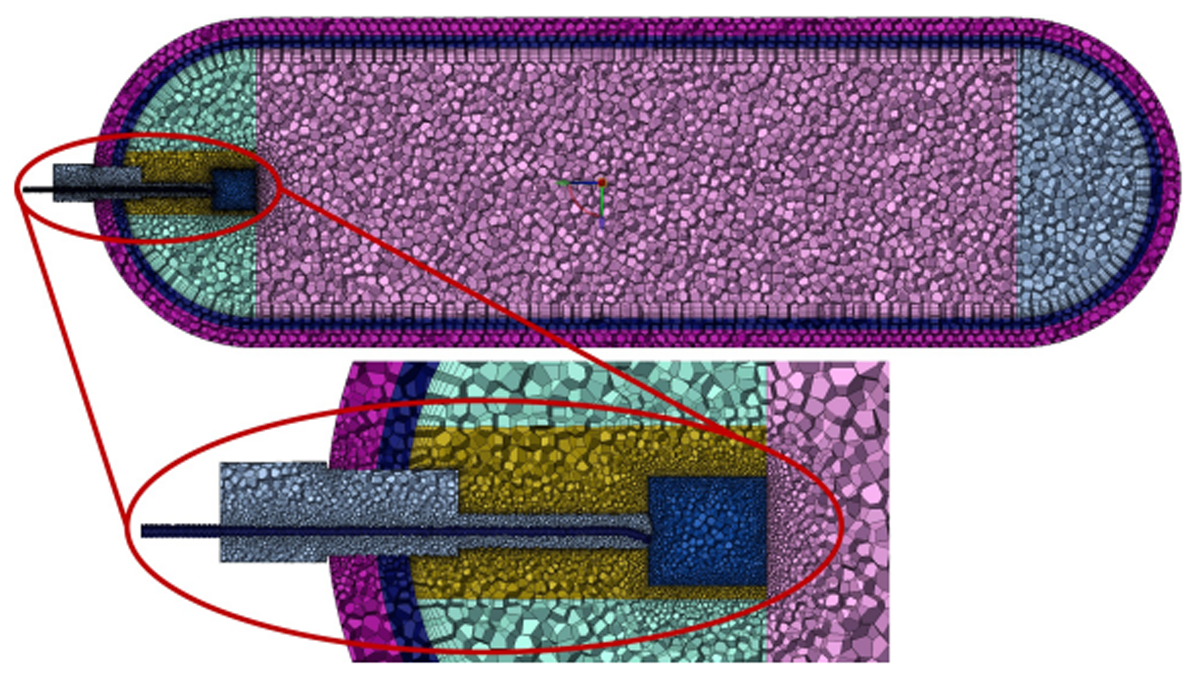
Figure 4
Computational mesh with local refinements.
Material properties for the fluid and solid zones were designated as per Figure 3. The Redlich-Kwong real gas model was applied for hydrogen, while material data for the aluminum valve, inner liner (Type III: aluminum or Type IV: high density polyethylene (HDPE)), and the composite (carbon-fiber reinforced polymer (CFRP)) outer layer followed specifications from Table 3. The properties of the solid materials were assumed to be constant for simplicity, and did not vary with temperature.
Table 3
Material properties (Bourgeois et al., 2018; Li et al., 2019).
| TYPE III | TYPE IV | |||
|---|---|---|---|---|
| LINER | OUTER LAYER | LINER | OUTER LAYER | |
| Material | Aluminum | CFRP | HDPE | CFRP |
| Density [kg/m3] | 2700 | 1494 | 947 | 1600 |
| Specific heat capacity [J/K/kg] | 900 | 938 | 1880 | 1400 |
| Thermal conductivity [W/k/m] | 202 | 1 | 0.3 | 1.5 |
A pressure-inlet type boundary condition (BC) was selected at the inlet, where the hydrogen pressure and temperature profiles were defined based on measurements taken just before the hydrogen entered the tank. While the pressure-inlet BC is widely used according to the literature for tank filling, some studies opt for a mass-flow inlet type BC instead (Li et al., 2019). On the valve and composite layer’s outer walls, a convective heat flux BC was implemented, setting the ambient free stream temperature (6°C for Tank A, 15°C for Tank C), which reflects the actual ambient conditions during the tests. The heat transfer coefficient was set at 8 W/m2/K, a value typical for still air (Klopčič et al., 2024).
The model includes several fluid-solid and solid-solid interfaces between adjacent domains, employing a coupled wall option where heat transfer (convection at fluid-solid, conduction at solid-solid) occurs between two neighboring cells from different domains. Additionally, a no-slip condition ensures zero fluid velocity at the fluid-solid interface. The initial conditions were set to mirror the experimental setup’s start: the tank was in thermal equilibrium with the surrounding environment at the respective ambient temperature, and an initial pressure of 30 bar in the case of Tank A and 5 bar for Tank C.
Choosing the most appropriate turbulence model remains a challenge; different models such as SST k-ω, variants of k-ϵ, or Reynolds Stress Models are considered (Bourgeois et al., 2018; Suryan, Kim and Setoguchi, 2013; Li et al., 2019; Ren, Lodier and Ammouri, 2023). This work initially used the realizable k-ϵ model due to its lower computational cost and an acceptable temperature deviation of less than 2°C as shown by Suryan, Kim, and Setoguchi (2013). However, more recent findings by Gonin et al. (2023a) suggest that the k-ω SST SAS model is superior for capturing thermal stratification, despite its higher computational demands. Both SST k-ω and k-ϵ models tend to overestimate thermal diffusion and thus underestimate thermal gradients (Martin et al., 2023; Gonin et al., 2023a). Given the already high computational intensity of refueling simulations, advanced turbulence models like Large Eddy Simulation (LES) are impractical (Martin et al., 2023).
Transport variables such as density, velocity, and temperature are stored at the centroids of volume cells, requiring discretization schemes for calculations at cell walls. A second-order upwind scheme was applied to all transport equations, as well as coupled pressure-velocity method. The simulation’s time step size was determined through a study that compared the first five seconds of the refueling process at different time steps, ranging from 0.0001 to 0.01 seconds. A time step of 0.001 seconds was selected as it provided sufficiently accurate results without further increasing computational costs. Larger time steps failed to meet the convergence criteria, resulting in decreasing tank temperatures instead of the expected increase. The continuity residual limit had to be reduced from the standard 1e-3 to 1e-6 to accurately reflect the expected increase in tank temperatures during refueling.
Overall, the required time for each simulation case exceeded a month of real-time computation on a server, where 16 cores were available for use for simulations with Tank A and 48 for Tank C.
3.0 results
3.1 Experimental
Experimental results – Tank A
The measured tank temperatures and pressure of the three experiments with Tank A are shown in Figure 5. The temperatures T1 to T5 correspond to the different measuring points on the lance. As seen from the figure, T5 is the sensor nearest to the hydrogen inlet, whereas T1 is the farthest, being at the opposite tank end. Starting with the horizontal filling case, it can be seen that sensors T1–T4 show nearly identical temperatures, whereas T5 is slightly lower due to being closer to the inflowing cold hydrogen. The final tank temperatures were measured at around 40°C. This shows that for shorter tanks filled horizontally, the temperature gradient in axial direction is small to negligible. However, it is also known from the literature that for such tanks, the hot spots usually occur above the OTV (Li et al., 2012). Additional temperature sensors placed in radial direction would have been helpful; however, due to the required modifications to the existing measuring probe, it was not feasible in the available timespan.
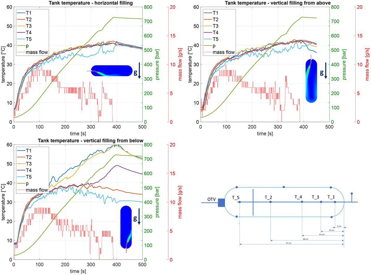
Figure 5
Experimental results of Tank A.
The experimental results of the horizontal case are similar to vertical filling from above, with temperatures in the axial direction again being nearly identical. This can be explained by the tendency of hotter gas to rise due to buoyancy being counteracted with the cold hydrogen entering from the top. The temperatures are 40°C as for the horizontal case.
In contrast, vertical filling from below shows a significant temperature gradient. For the first two minutes of the filling process, all temperatures were similar until the temperatures measured at T1 and T3 increased significantly. The most likely reason for this behavior lies in the decrease in flow velocity of the inflowing hydrogen jet. After reaching its maximum (approx. 10 g/s) around the 110 s mark, the mass flow starts to decrease. The density increase at higher pressures also leads to a decrease in flow velocity. Due to this, the hydrogen jet no longer penetrates until the upper part of the tank, causing the hot spot to form, and is additionally expedited by the buoyancy effects. Both the sensors T1 and T3 exhibit a maximum temperature of 60°C at the end of filling, indicating a larger, hotter zone at the top of the tank. Sensors T2 (placed at one-third tank length from the hydrogen inlet) and T4 (three-fifths tank length from inlet) measure similar temperatures until the 300 s mark, after which point the temperature at T4 increases until reaching 50°C. Around the time of T4 increasing, the temperatures of T2 and T5 start to decrease and are 35°C and 30°C respectively at the end of filling. The temperature delta between the sensors T1 and T5 is thus 30°C at the end of the filling process. Relying on the temperature measurement at the OTV could be a fatal mistake in such tank filling situations.
Experimental results – Tank B
For the nine tests with Tank B (all horizontal fillings), the temperature was recorded at the OTVs installed at the tank front (hydrogen inlet) and at the tank back end. Figure 6 shows the comparison of the calculated average temperature and the measured temperatures at both sensors inside the tank.
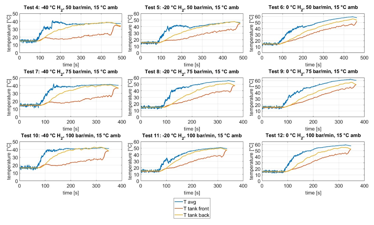
Figure 6
Experimental results of Tank B. Adapted from (Klopčič et al., 2024) according to CC-BY-4.0.
The measured sensor temperatures exhibit a significantly slower, near-linear increase compared to the exponential trend of the average temperature in the initial refueling phase. This results in lower recorded temperatures. Additionally, a notable temperature gradient along the tank axis is observed, with the front being cooler due to incoming hydrogen, while the back experienced higher temperatures. Similar findings were reported by Li et al. (2012) through 3D CFD simulations of large-tank refueling (~150 L, 1600 mm). These gradients arise from complex flow fields and circulation areas that induce temperature inhomogeneity.
The tests 4–12 demonstrate comparable temperature differences at the tank ends and relatively similar curve trends. Notably, the initial quarter of refueling showed minimal temperature variation across –40, –20, and 0°C hydrogen inlet conditions due to the cooling unit’s delay caused by thermal inertia. The front-to-back temperature difference reaches up to 10°C, highlighting that sensors at the OTV in commercial vehicle systems significantly underestimate average or peak tank temperatures during refueling.
As the average tank temperature is evidently higher than any individual sensor reading, hotter regions within the tank exist. However, direct calculation of the peak temperature from measurements is infeasible due to unknown temperature distributions and region sizes. In the final third of refueling, the differences between average temperature and the temperature at the back of the tank decrease to 3–5°C, or in some tests (no. 4, 5, 7, 10, 11), becomes negligible. By incorporating a safety margin, the measurement at the backside of the tank is able to approximate the average tank temperature. The sensor at the front, positioned near the cold hydrogen inlet, records lower temperatures. Only after the refueling stops does the front temperature rapidly rise and align with the back temperature.
Experimental results – Tank C
In Figure 7, the two measured tank temperatures, the tank pressure and the calculated average temperature (as described at the end of Section 2.1) are shown for the three test cases of Tank C. For the 5 min 5–438 bar filling, the process had to be stopped at around 300 bar tank pressure due to the temperature sensors reaching the 85°C limit. However, it can be seen that both sensors measured a significantly lower temperature than the expected average. This means that temperatures in the tank were even higher, up to 95°C in the aforementioned tests, posing a safety risk. Upon discussion with the manufacturer, a factor for the underprediction of the sensor could lie in the tank boss geometry. The neck of the boss is relatively long; thus, the temperature sensor may not have reached into the inner tank. Consequently, the tank boss geometry and OTV pairing potentially influence the temperature measurement.
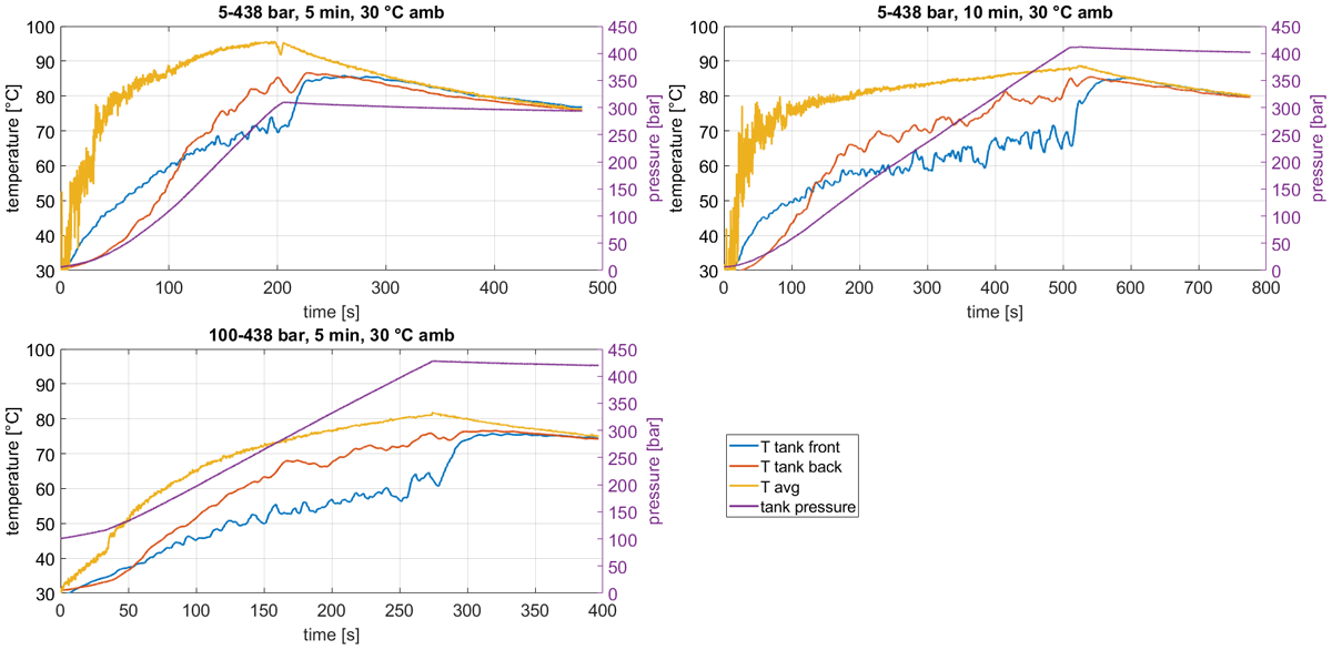
Figure 7
Experimental results of Tank C.
3.2 Simulation
Simulation results – Tank A
The average tank temperature was calculated as previously described and is compared with the volume-averaged temperature from simulations (Figure 8, left). Initially, both match closely for the first 20 seconds. However, especially from 20 to 50 s, the simulation underpredicts the temperature. After 50 s, the gradient of the temperature increase is greater in simulation, before converging with experimental results in the final third of refueling. The deviation in the first two-thirds cannot be attributed to a single cause but likely results from mass-pressure-temperature interactions via the thermodynamic equation of state and model settings (Bourgeois et al., 2018). The discrepancy likely stems from pressure loss through the OTV, as the simulation uses a simplified nozzle geometry due to a lack of exact design data. Consequently, pressure losses may differ from experimental conditions, resulting in an offset in tank mass. A mass-flow inlet boundary condition could improve predictions.
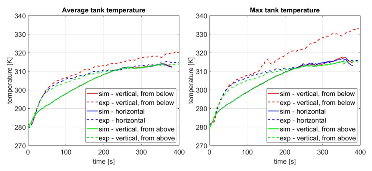
Figure 8
Comparison of average and maximum temperature between experiment and simulation of Tank A.
For comparison of the maximum temperature, the highest of the five measured values is selected, though it likely underestimates the true peak temperature. This is especially for the horizontal tank, where hot spots are above the valve (Li et al., 2012), making direct measurement challenging. The maximum temperature from the simulation follows trends similar to the average temperature (Figure 8, right) and is only slightly higher than the average. The vertical filling from above and horizontal tests show good agreement with the measured values. However, it must be noted again that for the horizontal tank, the highest measured temperature is not the actual highest temperature in the tank. For bottom refueling, the simulation significantly underpredicts the top sensor temperature due to the realizable k-ϵ model’s limitations in stratification. According to recent work by Gonin et al. (2023a), the k-ω SST SAS model should be adopted for improved accuracy.
Temperature distribution (Figure 9) is shown within a 300–317 K range to enhance clarity. The bottom refueling case shows a hot spot at the tank’s top, while in horizontal refueling, it forms just above the valve in the first half of the tank, consistent with findings for smaller tanks. In horizontal cases, the tank is short enough for cold hydrogen to flow along the wall, cooling the second tank half. In contrast, in topside refueling, rising hot gas is cooled by incoming hydrogen, resulting in a more uniform temperature distribution. It can thus be derived, that for vertical tank placement, the refueling should be topside. Despite discrepancies in absolute values, qualitatively the CFD results match with the experimental results.
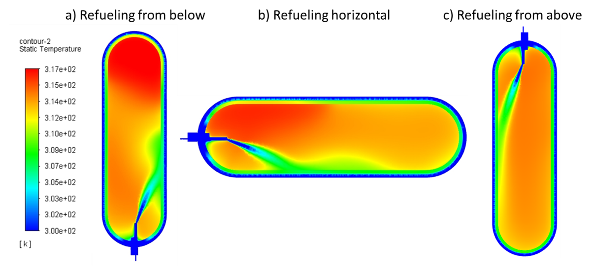
Figure 9
Simulated temperature distribution of the three filling cases of Tank A.
Simulation results – Tank C
The average tank temperature from 3D CFD simulations of Tank C is compared to the average temperature calculated based on experimental data in Figure 10. The CFD underpredicts at the beginning and overpredicts toward the end of the filling process. The deviation is expected to be mostly due to exact material properties and wall thickness not being provided by the manufacturer; thus, assumptions had to be made based on the literature data for Type IV tanks (Bourgeois et al., 2018; Li et al., 2019). However, the CFD results reconfirm that the two measurement locations greatly underpredict the actual tank temperatures. Therefore, relying on the temperature measurement at the OTV for the development of filling protocols could pose a significant safety risk.
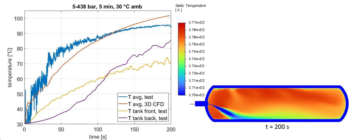
Figure 10
Comparison of simulated average tank temperature with experiments (left) and temperature distribution (right).
4.0 Conclusions
This work combines experimental tests with 3D CFD analyses on three different tanks. The findings reveal that the tanks exhibit inhomogeneous temperature distributions and that the standard temperature sensor integrated into the OTV can significantly underpredict the actual tank temperature. Relying solely on this sensor for developing filling protocols or for communication with filling stations could pose a safety risk.
While employing multiple, spatially distributed sensors would improve temperature mapping, such elaborate setups are too costly for large-scale applications. In-depth experiments and detailed 3D CFD simulations are necessary to accurately identify hot spot locations, but are expensive and time-consuming, making them impractical for evaluating every tank variant under diverse operating conditions. Consequently, simplified 0D model approaches must be developed for rapid parameter studies of filling processes. Ideally, a synergistic combination of 0D simulations, 3D CFD analyses, and experimental methods should be employed.
Although the CFD simulations successfully identified hot spot locations, they underestimated the temperature magnitudes in these regions. Future modeling efforts will prioritize turbulence model refinements—specifically by adopting the k-ω SST SAS or Reynolds Stress model—to better capture buoyancy effects. Additionally, a measuring lance equipped with extra sensors is currently under development for further tests with Tank C, and alternative, more reliable temperature measurement methods should be explored for practical applications. By combining further testing and validated simulations, a general methodology for accurate predictions in practical applications can be derived.
Competing Interests
The authors have no competing interests to declare.
Author Contributions
Nejc Klopčič – writing lead, design and conceptualization, simulation, experiments, data analysis, interpretation, supervision
Thomas Hafner – experimental setup, experiments, data analysis
Dominik Schiffer – simulation, data analysis, writing review
Patrick Pertl – interpretation, supervision, writing review
Alexander Trattner – supervision, funding acquisition, resources