Analysis of a Mechanistic Model for Non-invasive Bioimpedance of Intact Skin

We start with the mathematical model for EIS measurements derived by Birgersson et al. [12], which treats the skin as a three-layer entity: stratum corneum (SC) as the outermost layer characterized by corneocytes; viable skin (VS) consisting of both living epidermis and dermis; and adipose tissue (AT) to account for the subcutis layer containing a high percentage of fat, as illustrated in Fig. 1a-b While the non-invasive EIS probe in the studies by Birgersson et al. [12] comprised four electrodes – one current detector (sense), one guard and two injects – we will here consider a simpler probe with similar dimensions but only one current detector (at I) and one voltage injector (at II). The dimensions and material properties of the electrodes and skin layers can be found in Table 1.

Fig.1

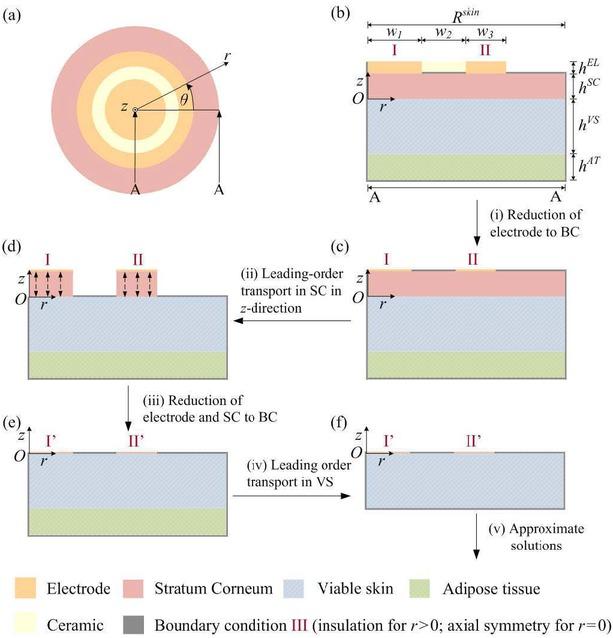
Schematic overview of the non-invasive two-electrode EIS probe and adjacent stratum corneum, viable skin and adipose tissue (a-b). The model reduction from the scaling analysis is illustrated in b-f.

Tab. 1

Current detection width, w1	2 mm
Ceramic width, w2	1.2 mm
Inject width, w3	1 mm
Outer radius of the probe, R	4.2 mm
Outer radius of the skin, Rskin	10 mm
Electrode thickness, hEL	0.1 mm	[18]
Stratum corneum thickness, hSC	14 μm	[18]
Viable skin thickness, hVS	1.2 mm	[18]
Adipose tissue thickness, hAT	1.2 mm	[18]
Inject voltage, V0	0.05 V
Electrical permittivity in vacuum, ɛ0	8.85 x107	[19]
	Fm-1
Relative permittivity of electrodes,	1	[20]
εrEL${{\varepsilon }_{r}}^{EL}$
Electrode conductivity, σEL	4.56 x107	[20]
	Sm-1

The mathematical model can be written as

(1)∇⋅J(r)=0,$$\nabla \cdot \mathbf{J}\left( \mathbf{r} \right)=0,$$

(2)Jr=−σeffk∇Φr,$$\mathbf{J}\left( \mathbf{r} \right)=-\sigma _{eff}^{k}\nabla \Phi \left( \mathbf{r} \right),$$

(3)Φ(I)=0,$$\Phi \left( \text{I} \right)=0,$$

(4)Φ(II)=V0,$$\Phi \left( \text{II} \right)={{V}_{0}},$$

(5)J(III)⋅n=0.$$\mathbf{J}\left( \text{III} \right)\cdot \mathbf{n}=0.$$

Here, the complex-valued phasors, Φ(r) and J(r) , for the potential and current density are functions of space only (although we note that they can be pulled back into the time domain), _n is the unit normal vector pointing outwards to any given boundary, V₀ is the applied voltage, and the location of the boundary conditions is given by roman numerals, see Fig. 1 for their location; the effective conductivity, σeffk,$\sigma _{eff}^{k},$is given by

(6)σeffk=σk+iωε0εrk,$$\sigma _{eff}^{k}={{\sigma }^{k}}+i\omega {{\varepsilon }_{0}}\varepsilon _{r}^{k},$$

where σ ^k is the electric conductivity, ε₀ and εrk$\varepsilon _{r}^{k}$are the relative permittivities of vacuum and the material respectively, i is the imaginary unit, and ω = 2πν is the angular frequency. The superscript, k, denotes either viable skin, stratum corneum soaked with a saline solution with 0.9% NaCl for 1 min, adipose tissue, or the electrode.

The material properties for the three skin layers on the volar forearm are defined as follows [17]:

(7)σk(N)=10−(c5kN5+c4kN4+c3kN3+c2kN2+c1kN+c0k),$${{\sigma }^{k}}\left( N \right)={{10}^{-\left( \mathbf{c}_{5}^{k}{{N}^{5}}+\mathbf{c}_{4}^{k}{{N}^{4}}+\mathbf{c}_{3}^{k}{{N}^{3}}+\mathbf{c}_{2}^{k}{{N}^{2}}+\mathbf{c}_{1}^{k}N+\mathbf{c}_{0}^{k} \right)}},$$

(8)εrk(N)=10(∂5kN5+∂4kN4+∂3kN3+∂2kN2+∂1kN+∂0k),$$\varepsilon _{r}^{k}\left( N \right)={{10}^{\left( \partial _{5}^{k}{{N}^{5}}+\partial _{4}^{k}{{N}^{4}}+\partial _{3}^{k}{{N}^{3}}+\partial _{2}^{k}{{N}^{2}}+\partial _{1}^{k}N+\partial _{0}^{k} \right)}},$$

(9)N=log10(v˜)$$N=\log 10\left( \widetilde{v} \right)$$

Here, cjk$\mathfrak{c}_{j}^{k}$and djk$\mathfrak{d}_{j}^{k}$are the material coefficients, given in Table 2; v˜=v/(1Hz$\widetilde{v}={v}/{\left( \text{1}\,\text{Hz} \right.}\;$is a dimensionless frequency and N is the uppercase greek letter of ν , introduced for notational convenience. These constitutive relations for the electrical material properties are valid between 1 kHz and 1 MHz; see Birgersson et al. [17] for the validation of these relations for two studies comprising 26 and 120 volunteers respectively.

Tab. 2

j	cjSC${{\mathfrak{c}}_{j}}^{SC}$	djSC${{\mathfrak{d}}_{j}}^{SC}$
0	-1.1803×101	1.7570×101
1	2.1404×101	-1.7961×101
2	-9.9955×100	8.5278×100
3	2.2537×100	-2.0255×100
4	-2.5509×10-1	2.3953×10-1
5	1.1516×10-2	-1.1319×10-2
j	cjVS${{\mathfrak{c}}_{j}}^{VS}$	djVS${{\mathfrak{d}}_{j}}^{VS}$
0	2.3688×101	6.7610×101
1	-2.7471×101	-7.0466×101
2	1.2952×101	3.2847×101
3	-3.0088×100	-7.7649×100
4	3.4167×10-1	9.2429×10-1
5	-1. 5178×10-2	-4.4465×10-2
j	cjAT$\mathfrak{c}_{j}^{AT}$	djAT$\mathfrak{d}_{j}^{AT}$
0	1.7402×100	7.5844×100
1	0	8.3142×10-2
2	0	-7.7214×10-1
3	0	1.1797×10-1
4	0	-4.0926×10-4
5	0	-5.2423×10-4

The impedance is defined as

(10)Z=V0I,$$Z=\frac{{{V}_{0}}}{I},$$

with the total current measured at the sense, boundary I in Fig. 1b, defined as

(11)I=2π∫0w1J(I)⋅nrdr.$$I=2\pi \int\limits_{0}^{{{w}_{1}}}{\mathbf{J}\left( \text{I} \right)\cdot \mathbf{n}rdr}.$$

We will refer to this model as the complete model.

We define the following dimensionless variables and dimensionless numbers:

(12)r˜=rR,z˜=Zhk,Z˜=Z[J]AsenV0,$$\widetilde{r}=\frac{r}{R},\widetilde{z}=\frac{Z}{{{h}^{k}}},\,\widetilde{Z}=\frac{Z\left[ J \right]{{A}^{sen}}}{{{V}_{0}}},$$

(13)J~=JJ,Φ~=ΦV0,Θk=hkR,$$\widetilde{\mathbf{J}}=\frac{\mathbf{J}}{\left[ J \right]},\,\widetilde{\Phi }=\frac{\Phi }{{{V}_{0}}},{{\Theta }^{k}}=\frac{{{h}^{k}}}{R},$$

(14)Πk=ωε0εrkσk,Λ1=πR2Asen,Ξk=σkhSCσSCR.$${{\Pi }^{k}}=\frac{\omega {{\varepsilon }_{0}}\varepsilon _{r}^{k}}{{{\sigma }^{k}}},{{\Lambda }_{1}}=\frac{\pi {{R}^{2}}}{{{A}^{sen}}},{{\Xi }^{k}}=\frac{{{\sigma }^{k}}{{h}^{SC}}}{{{\sigma }^{SC}}R}.$$

Here, [ ] is the scale (absolute value), R = w₁ + w₂ + w₃ is the overall radius of the outer electrode (inject) and Asen=πw12${{A}^{sen}}=\pi w_{1}^{2}$is the area of the inner electrode (sense); we have taken the scale for the impedance as [Z]=V0/([J]Asen).$\left[ Z \right]={{{V}_{0}}}/{\left( \left[ J \right]{{A}^{sen}} \right)}\;.$The dimensionless number, Π^k , is the ratio of the displacement and ohmic current; Θ^k relates the height of a given skin layer to the overall length in the radial direction; Λ₁ arises in the non-dimensionalization of the total current measured at the sense; and Ξk${{\Xi }^{k}}$gives the ratio of the current flowing through skin layer k to the current flowing through stratum corneum in the z -direction – and will provide valuable quantification of where the currents flow later in the analysis. We note that at this moment, the scale for the current, [J], is unknown.

These dimensionless variables and numbers are substituted into the governing equations for each layer of the skin, which we shall consider separately. Between the different layers, we require continuity of the current density as well as potential – we do not explicitly state those boundary conditions in the coming analysis for the sake of brevity.

In the stratum corneum, we obtain the following dimensionless transport equations:

(15)ΘSCr˜∂∂r˜(r˜J˜r)+∂J˜z∂z˜=0,$$\frac{{{\Theta }^{SC}}}{\widetilde{r}}\frac{\partial }{\partial \widetilde{r}}\left( \widetilde{r}{{\widetilde{J}}_{r}} \right)+\frac{\partial {{\widetilde{J}}_{z}}}{\partial \widetilde{z}}=0,$$

where

(16)J˜r=−σSCV0[J]R(1+iΠSC)∂Φ∂r˜,$${{\widetilde{J}}_{r}}=-\frac{{{\sigma }^{SC}}{{V}_{0}}}{\left[ J \right]R}\left( 1+i{{\Pi }^{SC}} \right)\frac{\partial \Phi }{\partial \widetilde{r}},$$

(17)J˜z=−σSCV0[J]hSC(1+iΠSC)∂Φ˜∂z˜.$${{\widetilde{J}}_{z}}=-\frac{{{\sigma }^{SC}}{{V}_{0}}}{\left[ J \right]{{h}^{SC}}}\left( 1+i{{\Pi }^{SC}} \right)\frac{\partial \widetilde{\Phi }}{\partial \widetilde{z}}.$$

Here, Π^SC ~ 1, as can be inferred from Fig. 2, whence we can identify the current density scale, [J], from Eqs. 16 and 17 as

Fig.2

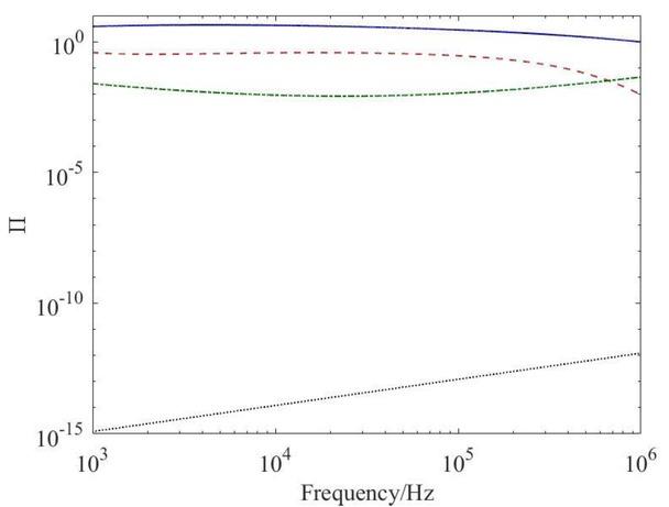
Dimensionless number, Π, for SC (–), VS (– –), AT (-⋅-) and EL (⋅⋅⋅).

[J]=σSCV0max(1R,1hSC)=σSCV0hSC.$$\left[ J \right]={{\sigma }^{SC}}{{V}_{0}}\max \left( \frac{1}{R},\frac{1}{{{h}^{SC}}} \right)=\frac{{{\sigma }^{SC}}{{V}_{0}}}{{{h}^{SC}}}.$$

Substituting the current density scale back into the governing equations, Eqs. 15, 16, 17, gives

(18)ΘSCr˜∂∂r˜(r˜J˜r)+∂J˜z∂z˜=0,$$\frac{{{\Theta }^{SC}}}{\widetilde{r}}\frac{\partial }{\partial \widetilde{r}}\left( \widetilde{r}{{\widetilde{J}}_{r}} \right)+\frac{\partial {{\widetilde{J}}_{z}}}{\partial \widetilde{z}}=0,$$

where

(19)J˜r=−ΘSC(1+iΠSC)∂Φ∂r˜,$${{\widetilde{J}}_{r}}=-{{\Theta }^{SC}}\left( 1+i{{\Pi }^{SC}} \right)\frac{\partial \Phi }{\partial \widetilde{r}},$$

(20)J˜z=−(1+iΠSC)∂Φ˜∂z˜.$${{\widetilde{J}}_{z}}=-\left( 1+i{{\Pi }^{SC}} \right)\frac{\partial \widetilde{\Phi }}{\partial \widetilde{z}}.$$

Furthermore, the stratum corneum is slender with

R ~10^-2 m and h^SC ~10^-5 m, such that

(21)ΘSC∼10−3≪1,$${{\Theta }^{SC}}\sim {{10}^{-3}}\ll 1,$$

and

(22)J˜z∼1,J˜r∼ΘSC≪1.$${{\widetilde{J}}_{z}}\sim 1,{{\widetilde{J}}_{r}}\sim {{\Theta }^{SC}}\ll 1.$$

In other words, the current density in the radial direction is around a thousand times smaller than the current in the z-direction for the conditions and probe dimensions considered here, whence Eq. 18 reduces to

(23)∂J˜z∂z˜=0,$$\frac{\partial {{\widetilde{J}}_{z}}}{\partial \widetilde{z}}=0,$$

subject to the boundary conditions adjacent to the electrodes

(24)Φ˜(I)=0,$$\widetilde{\Phi }\left( \text{I} \right)=0,$$

(25)Φ(II)=1,$$\Phi \left( \text{II} \right)=1,$$

and a continuous potential at the interface with the viable skin (N.B.: the potential drop in the electrodes is negligible at leading order as we shall show later). The current between the inject and the sense in the radial direction thus has to occur in the viable skin and/or adipose tissue, because the voltage is not enough to drive the current through the SC in the radial direction.

Returning to the current density scale for the frequency range of 1 kHz to 1 MHz that is of interest here, we find that

(26)[J]=σSCV0hSC∼10−2︸1kHz−10−1︸1kHzAm−2,$$\left[ J \right]=\frac{{{\sigma }^{SC}}{{V}_{0}}}{{{h}^{SC}}}\sim \underbrace{{{10}^{-2}}}_{1\,\text{kHz}}-\underbrace{{{10}^{-1}}}_{1\,\text{kHz}}\,\text{A}{{\text{m}}^{-\text{2}}},$$

which provides the scale for the current density in the z-direction for the base-case parameters and conditions; in the radial direction, the scale for current density is [J]ΘSC∼10−5−10−2Am-2$\left[ J \right]{{\Theta }^{SC}}\sim {{10}^{-5}}-{{10}^{-2}}\,\,\text{A}\,{{\text{m}}^{\text{-2}}}$We verify these scales with the numerical solution in the stratum corneum for 1 kHz to 1 MHz, which gives |Jr|∼10−6−10−2Am-2,$\left| {{J}_{r}} \right|\sim {{10}^{-6}}-{{10}^{-2}}\,\text{A}\,{{\text{m}}^{\text{-2}}},$evaluated at r=w1+w2/2,0<z<hSC,$r={{w}_{1}}+{{{w}_{2}}}/{2}\;,\,\,\,0<z<{{h}^{SC}},$which is between the two electrodes; and |Jz|∼10−2−10Am-2,$\left| {{J}_{z}} \right|\sim {{10}^{-2}}-10\,\,\text{A}\,{{\text{m}}^{\text{-2}}},$evaluated at 0 < r < w₁, z = h^SC , which is underneath the sense.

Finally, we confirm that scaling the potential, Φ˜=Φ/V0,$\widetilde{\Phi }={\Phi }/{{{V}_{0}},}\;$in the stratum corneum with V₀ in the entire frequency range is correct by comparing with the numerical simulations of the absolute voltage drop underneath the sense (r=w1/2,0≤z≤hSC)$\left( r={{{w}_{1}}}/{2,0\le z\le {{h}^{SC}}}\; \right)$and the inject (r=w1+w2+w3/2,0≤z≤hSC),$\left( r={{{w}_{1}}+{{w}_{2}}+{{w}_{3}}}/{2,0\le z\le {{h}^{SC}}}\; \right),$which are around 0.033 – 0.024 V and 0.017 – 0.013 V respectively for 1 kHz to 1 MHz. These voltage drops are indeed O(V₀ ). The higher

potential drop underneath the sense compared to the inject originates from the fact that the area of the inject is roughly two times larger than the sense for the base case conditions.

For the viable skin,

(27)ΘVSr˜∂∂r˜(r˜J˜r)+∂J˜z∂z˜=0,$$\frac{{{\Theta }^{VS}}}{\widetilde{r}}\frac{\partial }{\partial \widetilde{r}}\left( \widetilde{r}{{\widetilde{J}}_{r}} \right)+\frac{\partial {{\widetilde{J}}_{z}}}{\partial \widetilde{z}}=0,$$

where

(28)J˜r=−ΞVS(1+iΠVS)∂Φ˜∂r˜,$${{\widetilde{J}}_{r}}=-{{\Xi }^{VS}}\left( 1+i{{\Pi }^{VS}} \right)\frac{\partial \widetilde{\Phi }}{\partial \widetilde{r}},$$

(29)J˜z=−ΞVSΘVS(1+iΠVS)∂Φ˜∂z˜,$${{\widetilde{J}}_{z}}=-\frac{{{\Xi }^{VS}}}{{{\Theta }^{VS}}}\left( 1+i{{\Pi }^{VS}} \right)\frac{\partial \widetilde{\Phi }}{\partial \widetilde{z}},$$

and

(30)ΘVS∼1,ΠVS<1.$${{\Theta }^{VS}}\sim 1,{{\Pi }^{VS}}<1.$$

In order for the current to be carried through the viable skin between the inject and the sense, we require that ΞVS∼${{\Xi }^{VS}}\sim $1 in Eqs. 28 and 29 for both the left-hand and righthand sides to be O(1), which is not the case since

(31)100(1kHz)≳ΞVS≳1(1MHz),$$100\left( 1\text{kHz} \right)\gtrsim {{\Xi }^{VS}}\gtrsim 1\,\left( 1\,\,\text{MHz} \right),$$

as illustrated in Figure 3.

Fig.3

Dimensionless number, Ξ$\Xi $Ξ, for SC (–), VS (– –), AT (-⋅-) and EL (⋅⋅⋅).

This in turn suggests that we need to revisit the potential drop in the viable skin, which we assumed to be ~ V₀ when we scaled Φ = Φ / V₀ . If we rescale the potential,

(32)Φ^=Φ˜V0ΔΦVS,$$\widehat{\Phi }=\frac{\widetilde{\Phi }{{V}_{0}}}{\Delta {{\Phi }^{VS}}},$$

with ΔΦ^VS denoting an as-of-yet unknown scale for the potential drop, Eqs. 27, 28, 29 take the form

(33)ΘVSr˜∂∂r˜(r˜J˜r)+∂J˜z∂z˜=0,$$\frac{{{\Theta }^{VS}}}{\widetilde{r}}\frac{\partial }{\partial \widetilde{r}}\left( \widetilde{r}{{\widetilde{J}}_{r}} \right)+\frac{\partial {{\widetilde{J}}_{z}}}{\partial \widetilde{z}}=0,$$

with

(34)J˜r=−ΞVSΔΦVSV0(1+iΠVS)∂Φ^∂r˜,$${{\widetilde{J}}_{r}}=-{{\Xi }^{VS}}\frac{\Delta {{\Phi }^{VS}}}{{{V}_{0}}}\left( 1+i{{\Pi }^{VS}} \right)\frac{\partial \widehat{\Phi }}{\partial \widetilde{r}},$$

(35)J˜r=−ΞVSΘVSΔΦVSV0(1+iΠVS)∂Φ^∂z˜.$${{\widetilde{J}}_{r}}=-\frac{{{\Xi }^{VS}}}{{{\Theta }^{VS}}}\frac{\Delta {{\Phi }^{VS}}}{{{V}_{0}}}\left( 1+i{{\Pi }^{VS}} \right)\frac{\partial \widehat{\Phi }}{\partial \widetilde{z}}.$$

Again, we require that J˜r∼J˜z∼(N.B.ΘVS∼1)${{\widetilde{J}}_{r}}\sim {{\widetilde{J}}_{z}}\sim \left( \text{N}\text{.B}\text{.}\,\,\,\,{{\Theta }^{VS}}\sim 1 \right)$for the current to be carried through the viable skin, i.e.

(36)ΞVSΔΦVSV0∼1,$${{\Xi }^{VS}}\frac{\Delta {{\Phi }^{VS}}}{{{V}_{0}}}\sim 1,$$

which gives the scale for the potential drop,

(37)ΔΦVS∼V0ΞVS.$$\Delta {{\Phi }^{VS}}\sim \frac{{{V}_{0}}}{{{\Xi }^{VS}}}.$$

For the base case,

(38)10−4V︸1kHz≲ΔΦVS≲10−4V︸1MHz∼V0,$$\underbrace{{{10}^{-4}}\,V}_{1\,\text{kHz}}\lesssim \Delta {{\Phi }^{VS}}\lesssim \underbrace{{{10}^{-4}}\,V}_{1\,\text{MHz}}\sim {{V}_{0}},$$

which agrees well with the numerical solutions of the complete model (not shown here).

For the adipose tissue,

(39)ΘATr˜∂∂r˜(r˜J˜r)+∂J˜z∂z˜=0,$$\frac{{{\Theta }^{AT}}}{\widetilde{r}}\frac{\partial }{\partial \widetilde{r}}\left( \widetilde{r}{{\widetilde{J}}_{r}} \right)+\frac{\partial {{\widetilde{J}}_{z}}}{\partial \widetilde{z}}=0,$$

where

(40)J˜r=−ΞAT(1+iΠAT)∂Φ˜∂r˜,$${{\widetilde{J}}_{r}}=-{{\Xi }^{AT}}\left( 1+i{{\Pi }^{AT}} \right)\frac{\partial \widetilde{\Phi }}{\partial \widetilde{r}},$$

(41)J˜z=−ΞATΘAT(1+iΠAT)∂Φ˜∂z˜,$${{\widetilde{J}}_{z}}=-\frac{{{\Xi }^{AT}}}{{{\Theta }^{AT}}}\left( 1+i{{\Pi }^{AT}} \right)\frac{\partial \widetilde{\Phi }}{\partial \widetilde{z}},$$

and

(42)ΘAT∼1.$${{\Theta }^{AT}}\sim 1.$$

Now, because

(43)ΠAT∼10−2≪1,$${{\Pi }^{AT}}\sim {{10}^{-2}}\ll 1,$$

the current in the adipose tissue is mainly ohmic, such that we can write

(44)J˜r=−ΞAT∂Φ˜∂r˜,$${{\widetilde{J}}_{r}}=-{{\Xi }^{AT}}\frac{\partial \widetilde{\Phi }}{\partial \widetilde{r}},$$

(45)J˜z=−ΞATΘAT∂Φ˜∂z˜.$${{\widetilde{J}}_{z}}=-\frac{{{\Xi }^{AT}}}{{{\Theta }^{AT}}}\frac{\partial \widetilde{\Phi }}{\partial \widetilde{z}}.$$

For the current to be carried through the adipose tissue, we require that ΞAT∼1;${{\Xi }^{AT}}\sim 1;$returning to Fig. 3, however, we see that ΞAT∼20−2×10−2${{\Xi }^{AT}}\sim 20-2\times {{10}^{-2}}$at 1 kHz and 1 MHz respectively.

Rescaling the potential drop like what we did for the viable skin,

(46)Φ^=V0ΔΦATΦ˜,$$\widehat{\Phi }=\frac{{{V}_{0}}}{\Delta {{\Phi }^{AT}}}\widetilde{\Phi },$$

and requiring J˜r∼J˜z∼1(N.B.ΘAT∼1)${{\widetilde{J}}_{r}}\sim {{\widetilde{J}}_{z}}\sim 1\left( N.B.\,\,{{\Theta }^{AT}}\sim 1 \right)$i.e.

(47)ΞATΔΦATV0∼1,$${{\Xi }^{AT}}\frac{\Delta {{\Phi }^{AT}}}{{{V}_{0}}}\sim 1,$$

we find the scale for the potential drop in the adipose tissue,

(48)ΔΦAT∼V0ΞAT.$$\Delta {{\Phi }^{AT}}\sim \frac{{{V}_{0}}}{{{\Xi }^{AT}}}.$$

With the base case parameters,

(49)3×10−3V︸1kHZ≲ΔΦAT≲2.4V︸1MHz.$$\underbrace{3\times {{10}^{-3}}V}_{1\,\text{kHZ}}\lesssim \Delta {{\Phi }^{AT}}\lesssim \underbrace{2.4\text{V}}_{1\,\text{MHz}}.$$

Clearly, the current from the probe cannot be carried through the adipose tissue at 1 MHz since it would require around forty times the applied voltage, V₀; at the other end of the considered spectrum, 1 kHz, the voltage drop in the adipose tissue is around ten times larger than that of the viable skin; i.e.

(50)ΔΦATΔΦVS∼ΞVSΞAT∼10(1kHZ)−50(1MHz).$$\frac{\Delta {{\Phi }^{AT}}}{\Delta {{\Phi }^{VS}}}\sim \frac{{{\Xi }^{VS}}}{{{\Xi }^{AT}}}\sim 10\left( 1\,\text{kHZ} \right)-50\left( 1\,\text{MHz} \right).$$

In other words, most of the current from the inject would choose the easier path through the viable skin before even going deeper through the viable skin to reach the adipose tissue, after which the current would need to pass through the adipose tissue in the radial direction and then upwards through the viable skin again.

In the electrodes, the dimensionless governing equations can be written as

(51)ΘELr˜∂∂r˜(r˜J˜r)+∂J˜z∂z˜=0,$$\frac{{{\Theta }^{EL}}}{{\tilde{r}}}\frac{\partial }{\partial \tilde{r}}\left( \tilde{r}{{{\tilde{J}}}_{r}} \right)+\frac{\partial {{{\tilde{J}}}_{z}}}{\partial \tilde{z}}=0,$$

where

(52)J˜r=−ΞEL(1+i∏EL)∂Φ˜∂r˜,$${{\tilde{J}}_{r}}=-{{\Xi }^{EL}}\left( 1+i\prod{^{EL}} \right)\frac{\partial \tilde{\Phi }}{\partial \tilde{r}},$$

(53)J˜z=−ΞELΦEL(1+i∏EL)∂Φ˜∂z˜.$${{\tilde{J}}_{z}}=-\frac{{{\Xi }^{EL}}}{{{\Phi }^{EL}}}\left( 1+i\prod{^{EL}} \right)\frac{\partial \tilde{\Phi }}{\partial \tilde{z}}.$$

Because Π^EL ~ 10^-15 -10^-12 ≪ 1, the displacement current is negligible compared to the ohmic counterpart in the electrodes; in addition, ΞEL~1011−108${{\Xi }^{EL}}\tilde{\ }{{10}^{11}}-{{10}^{8}}$for 1 kHz to 1 MHz, which implies that the voltage drop in the electrodes is negligible compared to the drop across the skin layers. There is thus no need to consider the potential drop in the electrodes.

Now that we have analyzed the currents in the electrodes and three skin layers in detail to deduce the leading-order phenomena, we can combine the findings to arrive at a reduced model, as illustrated in Fig. 1b-1f

In the first step from Fig. 1b to 1c, the electrodes do not need to be resolved due to the negligible potential drops in these; we can thus move the boundaries for the ground, I, and applied potential, II, down to the stratum corneum; i.e. at the sense (I),

(54)Φ(0≤r≤R1,z=hSC)=0,$$\Phi \left( 0\le r\le {{R}_{1}},z={{h}^{SC}} \right)=0,$$

and at the inject (II),

(55)Φ(R2≤r≤R3,z=hSC)=V0,$$\Phi \left( {{R}_{2}}\le r\le {{R}_{3}},z={{h}^{SC}} \right)={{V}_{0}},$$

where R₁ = w₁, R₂ = w₁ + w₂ , R₃ = w₁ + w₂ + w₃ (= R) for notational convenience.

In the second and third steps from Fig. 1c to 1e, the leading-order transport in the stratum corneum for the frequencies considered here is in the z-direction, whence the PDE reduces to an ordinary differential equation, which we can integrate analytically and so reduce this layer to the modified boundary conditions, I’and II’ adjacent to the viable skin. We can capture these two steps in our reduced model by returning to Eq. 23 and writing it in dimensional form as

(56)∂Jz(r,z)∂z=0,$$\frac{\partial {{J}_{z}}\left( r,z \right)}{\partial z}=0,$$

which gives us that J _z is constant in the z-direction in the stratum corneum (the radial component is O(Θ^SC ) ≪ 1 for the conditions we consider here); i.e., it is a function of r only. With the definition of the current density, we can write

(57)−σeffSC∂Φ(r,z)∂z=Jz(r),$$-\sigma _{eff}^{SC}\frac{\partial \Phi \left( r,z \right)}{\partial z}={{J}_{z}}\left( r \right),$$

which can be integrated once to give

(58)Φ(r,z)=−Jz(r)σeffSCz+C.$$\Phi \left( r,z \right)=-\frac{{{J}_{z}}\left( r \right)}{\sigma _{eff}^{SC}}z+C.$$

With the boundary condition, Eq. 55, underneath the inject, we can determine the integration constant, C, and write the potential as

(59)Φ(r,z)=Jz(r)σeffSC(hSC−z)+V0.$$\Phi \left( r,z \right)=\frac{{{J}_{z}}\left( r \right)}{\sigma _{eff}^{SC}}\left( {{h}^{SC}}-z \right)+{{V}_{0}}.$$

At the interface between the stratum corneum and viable skin (II'; z=0 in Eq. 59), we can now introduce the modified boundary condition in lieu of the stratum corneum and the inject as

(60)Jz(II’)=S(Φ−V0),$${{J}_{z}}\left( \text{II} \right)=S\left( \Phi -{{V}_{0}} \right),$$

where, again for convenience,

(61)S=σeffSChSC.$$S=\frac{\sigma _{eff}^{SC}}{{{h}^{SC}}}.$$

Returning to the sense (I) and the boundary condition, Eq. 54, we can repeat the integration above and write the modified boundary condition for the reduced model as

(62)Jz(I’)=SΦ.$${{J}_{z}}\left( I\text{} \right)=S\Phi .$$

In the fourth step from Fig. 1e to 1f, the contribution of the adipose tissue to the impedance is negligible at leading order, whence we do not need to resolve this layer.

After these four steps, we can finally formulate the dimensional governing equations and boundary conditions, because it is not necessary to go through the entire nondimensionalization to employ the model:

(63)∇⋅J=0,$$\nabla \cdot \mathbf{J}=0,$$

(64)J=−σeffVS∇Φ,$$\mathbf{J}=-\sigma _{eff}^{VS}\nabla \Phi ,$$

(65)J(I’)⋅n=SΦ,$$\mathbf{J}\left( \text{I} \right)\cdot \mathbf{n}=S\Phi ,$$

(66)J(II’)⋅n=S(Φ−V0),$$\mathbf{J}\left( \text{II} \right)\cdot \mathbf{n}=S\left( \Phi -{{V}_{0}} \right),$$

(67)J(III)⋅n=0,$$\mathbf{J}\left( \text{III} \right)\cdot \mathbf{n}=0,$$

(68)Zred=V0(2π∫0R1J(I’)⋅nrdr.)−1.$${{Z}_{red}}={{V}_{0}}{{\left( 2\pi \int\limits_{0}^{{{R}_{1}}}{\mathbf{J}\left( \text{I} \right)\cdot \mathbf{n}rdr}. \right)}^{-1}}.$$

We note that the initial boundary conditions – two Dirichlet and one Neuman condition – have been replaced by two Robin and one Neuman condition.

The reduced model – a Laplace equation with a Neuman and two Robin conditions – still requires a numerical method to solve. It is thus not as straight-forward to employ as equivalent circuits nor does it readily yield the functional form of the measured impedance and its dependence on the parameters. We therefore proceed with our analysis with a view to secure semi-analytical or analytical solutions (step v in Fig. 1). As we shall see, these solutions will be approximate in nature; i.e. we will make assumptions during the derivation.

Now, because we are primarily interested in the measured impedance (macroscopic, integral quantity) and not the pointwise potential distribution (microscopic quantity) throughout the electrodes and skin layers, we start by integrating the reduced model, Eqs. 63, 64, and invoking the divergence theorem,

(69)∫V∇⋅JdV=∮AJ⋅ndA=0,$$\int\limits_{V}{\nabla \cdot \mathbf{J}dV}=\oint\limits_{A}{\mathbf{J}\cdot \mathbf{n}dA}=0,$$

where V is the volume and A is the outer area bounding the volume.

Introducing the boundary conditions, Eqs. 65, 67, into the integral formulation, Eq. 69, gives

(70)AsenSΦsen︸=I+AinjS(Φinj−V0)︸=−I=0,$$\underbrace{{{A}^{sen}}S{{\Phi }^{sen}}}_{=I}+\underbrace{{{A}^{inj}}S\left( {{\Phi }^{inj}}-{{V}_{0}} \right)}_{=-I}=0,$$

where Ф^sen and Ф^inj are the area-averaged potentials at the sense and inject respectively:

(71)Φsen=2π∫0R1Φ(r,0)rdrAsen,$${{\Phi }^{sen}}=\frac{2\pi \int{_{0}^{{{R}_{1}}}\Phi \left( r,0 \right)r\,dr}}{{{A}^{sen}}},$$

(72)Φinj=2π∫R2R3Φ(r,0)rdrAinj$${{\Phi }^{inj}}=\frac{2\pi \int{_{{{R}_{2}}}^{{{R}_{3}}}\Phi \left( r,0 \right)r\,dr}}{{{A}^{inj}}}$$

Here, I is the total current and the areas of the sense and inject are

(73)Asen=πR12,$${{A}^{sen}}=\pi R_{1}^{2},$$

(74)Ainj=π(R32−R22).$${{A}^{inj}}=\pi \left( R_{3}^{2}-R_{2}^{2} \right).$$

Let us define the overall potential drop across the viable skin as

(75)ΔVVS=Φinj−Φsen,$$\Delta {{V}^{VS}}={{\Phi }^{inj}}-{{\Phi }^{sen}},$$

and argue based on linearity that ΔV ^VS should be a function of the current density, the effective conductivity of the viable skin and a representative average length for the current flowing through the viable skin, L; i.e.

(76)ΔVVS=IσeffVSL,$$\Delta {{V}^{VS}}=\frac{I}{\sigma _{eff}^{VS}L},$$

Assuming that we will later be able to quantify L, we now have four equations for our primary variables, Φ ^sen , Φ^inj , I, and Z:

(77)AsenSΦsen=I,$${{A}^{sen}}S{{\Phi }^{sen}}=I,$$

(78)AinjS(Φinj−V0)=−I,$${{A}^{inj}}S\left( {{\Phi }^{inj}}-{{V}_{0}} \right)=-I,$$

(79)Φinj−Φsen=IσeffVSL,$${{\Phi }^{inj}}-{{\Phi }^{sen}}=\frac{I}{\sigma _{eff}^{VS}\,L},$$

(80)Z=V0I.$$Z=\frac{{{V}_{0}}}{I}.$$

After some algebra, we find the current and impedance as

(81)I=AinjAsenSV0(1+ℭ)Asen+Ainj,$$I=\frac{{{A}^{inj}}{{A}^{sen}}S{{V}_{0}}}{\left( 1+\mathfrak{C} \right){{A}^{sen}}+{{A}^{inj}}},$$

(82)Z=1S(1Asen+1+ℭAinj),$$Z=\frac{1}{S}\left( \frac{1}{{{A}^{sen}}}+\frac{1+\mathfrak{C}}{{{A}^{inj}}} \right),$$

with

(83)ℭ=AinjSσeffVSL.$$\mathfrak{C}=\frac{{{A}^{inj}}S}{\sigma _{eff}^{VS}L}.$$

Returning to the definition of S in Eq. 61, we can express C as

(84)ℭ=AinjσeffSChSCσeffVSL,$$\mathfrak{C}=\frac{{{A}^{inj}}\sigma _{eff}^{SC}}{{{h}^{SC}}\sigma _{eff}^{VS}L},$$

which acts as a dimensionless correction factor for the current and impedance; i.e. if ℭ≪1$\mathfrak{C}\ll 1$we obtain

(85)I1=AinjAsenSV0Asen+Ainj,$${{I}_{1}}=\frac{{{A}^{inj}}{{A}^{sen}}S{{V}_{0}}}{{{A}^{sen}}+{{A}^{inj}}},$$

(86)Z1=1S(1Asen+1Ainj).$${{Z}_{1}}=\frac{1}{S}\left( \frac{1}{{{A}^{sen}}}+\frac{1}{{{A}^{inj}}} \right).$$

In particular, if we take A^inj ~ R² and L - R , we see that

(87)ℭ~RσSChSCσVS=1ΞVS~ΔΦVSΔΦSC,$$\mathfrak{C}\tilde{\ }\frac{R{{\sigma }^{SC}}}{{{h}^{SC}}{{\sigma }^{VS}}}=\frac{1}{{{\Xi }^{VS}}}\tilde{\ }\frac{\Delta {{\Phi }^{VS}}}{\Delta {{\Phi }^{SC}}},$$

based on the potential drops that were defined in the earlier analysis for the skin layers. The condition ℭ≪1$\mathfrak{C}\ll 1$thus corresponds to the scenario when the impedance is dominated by the stratum corneum, ΔΦ^VS ≪ ΔΦ^SC , which is typically the case for frequencies around 1 kHz. Noteworthy is that the closed-form solution for the impedance in Eq. 86 is identical to our analytical solution for a four-electrode probe around 1 kHz [13] when only considering two electrodes.

Let us now try to determine L and its functional form. For this purpose, we will carry out a Hankel transform of zeroth order, H₀ { Φ ( r , z ) } , similar to Cheng et al. [21],

Ψξ,z=H0Φr,z=∫0∞rΦr,zJ0ξrdr,$$\Psi \left( \xi ,z \right)=H_0\left\{ \Phi \left( r,z \right) \right\}=\int_{0}^{\infty }{r\Phi \left( r,z \right)}{{J}_{0}}\left( \xi r \right)dr,$$

because it allows us to transform our axisymmetric Laplace equation in cylindrical coordinates (Eq. 63),

(88)1r∂∂r(r∂Φ∂r)+∂2Φ∂z2=0,$$\frac{1}{r}\frac{\partial }{\partial r}\left( r\frac{\partial \Phi }{\partial r} \right)+\frac{{{\partial }^{2}}\Phi }{\partial {{z}^{2}}}=0,$$

to an ordinary differential equation,

H0{ΔΦ(r,z)}=−ξ2Ψ(ξ,z)+∂Ψ∂z2(ξ,z)=0,$${{H}_{0}}\left\{ \Delta \Phi \left( r,z \right) \right\}=-{{\xi }^{2}}\Psi \left( \xi ,z \right)+\frac{\partial \Psi }{\partial {{z}^{2}}}\left( \xi ,z \right)=0,$$

with the solution

(89)Ψ(ξ,z)=A(ξ)e−ξz+B(ξ)eξz,$$\Psi \left( \xi ,z \right)=A\left( \xi \right){{e}^{-\xi z}}+B\left( \xi \right){{e}^{\xi z}},$$

where A(ξ ) and B(ξ ) are two functions that we will soon determine from the transformed boundary conditions; J₀ is the 0^th-order Bessel function of the first kind and Δ is the Laplace operator. At this stage, we note that our transformed solution automatically satisfies the circular symmetry and requires that

(90)limr→∞Φ(r,z)=0,$$\underset{r\to \infty }{\mathop{\lim }}\,\Phi \left( r,z \right)=0,$$

which is reasonable since we expect the measured impedance to mainly be determined by the current flowing between the two electrodes; in fact, we have in the original boundary condition, Eq. 67, artificially limited the computational domain by assuming insulation for r = R^skin and choosing R^skin sufficiently large not to affect the impedance significantly.

If we further assume that the current across each electrode is constant, we can simplify Eqs. 65 and 66 to

(91)−σeffVS∂Φ(r,0)∂z=IπR12U(R1−r)−Iπ(R32−R22)[U(R3−r)−U(R2−r)],$$\begin{align}& -\sigma _{eff}^{VS}\frac{\partial \Phi \left( r,0 \right)}{\partial z}=\frac{I}{\pi R_{1}^{2}}U\left( {{R}_{1}}-r \right) \\ & -\frac{I}{\pi \left( R_{3}^{2}-R_{2}^{2} \right)}\left[ U\left( {{R}_{3}}-r \right)-U\left( {{R}_{2}}-r \right) \right], \\ \end{align}$$

or, after the Hankel transform,

−σeffVS∂Ψ(ξ,0)∂z=IπξR12R1J1(R1ξ)$$-\sigma _{eff}^{VS}\frac{\partial \Psi \left( \xi ,0 \right)}{\partial z}=\frac{I}{\pi \xi R_{1}^{2}}{{R}_{1}}{{J}_{1}}\left( {{R}_{1}}\xi \right)$$

(92)−Iπξ(R32−R22)[R3J1(R3ξ)−R2J1(R2ξ)],$$-\frac{I}{\pi \xi \left( R_{3}^{2}-R_{2}^{2} \right)}\left[ {{R}_{3}}{{J}_{1}}\left( {{R}_{3}}\xi \right)-{{R}_{2}}{{J}_{1}}\left( {{R}_{2}}\xi \right) \right],$$

where we have used that the Hankel transform of zeroth order of a Heaviside function, U(a - r) , is defined as

(93)H0{U(a−r)}=aξJ1(aξ),$${{H}_{0}}\left\{ U\left( a-r \right) \right\}=\frac{a}{\xi }{{J}_{1}}\left( a\xi \right),$$

with J₁ and a denoting the 1^st-order Bessel function of the first kind and a constant respectively. The remaining boundary condition, Eq. 67, becomes after transformation

(94)∂Ψ(ξ,−hVS)∂z=0.$$\frac{\partial \Psi \left( \xi ,-{{h}^{VS}} \right)}{\partial z}=0.$$

Substituting the z-derivative of the solution, Eq. 89,

(95)∂Ψ(ξ,z)∂z=−A(ξ)ξe−ξz+B(ξ)ξeξz,$$\frac{\partial \Psi \left( \xi ,z \right)}{\partial z}=-A\left( \xi \right)\xi {{e}^{-\xi z}}+B\left( \xi \right)\xi {{e}^{\xi z}},$$

into Eq. 94 gives

(96)A(ξ)=B(ξ)e−2ξhVS.$$A\left( \xi \right)=B\left( \xi \right){{e}^{-2\xi {{h}^{VS}}}}.$$

Proceeding to the other boundary condition, Eq. 91, we find after substituting the solution thus far,

(97)−σeffVS[B(ξ)ξ(1−e−2ξhVS)]=IπξR1J1(R1ξ)−Iπξ(R32−R22)[R3J1(R3ξ)−R2J1(R2ξ)],$$\begin{align}& -\sigma _{eff}^{VS}\left[ B\left( \xi \right)\xi \left( 1-{{e}^{-2\xi {{h}^{VS}}}} \right) \right]=\frac{I}{\pi \xi {{R}_{1}}}{{J}_{1}}\left( {{R}_{1}}\xi \right) \\ & \,\,\,\,\,-\frac{I}{\pi \xi \left( R_{3}^{2}-R_{2}^{2} \right)}\left[ {{R}_{3}}{{J}_{1}}\left( {{R}_{3}}\xi \right)-{{R}_{2}}{{J}_{1}}\left( {{R}_{2}}\xi \right) \right], \\ \end{align}$$

whence

(98)B(ξ)=Iκ(ξ)σeffVSξ(e−2ξhVS−1),$$B\left( \xi \right)=\frac{I\kappa \left( \xi \right)}{\sigma _{eff}^{VS}\xi \left( {{e}^{-2\xi {{h}^{VS}}}}-1 \right)},$$

and

(99)κ(ξ)=J1(R1ξ)πξR1−R3J1(R3ξ)−R2J1(R2ξ)πξ(R32−R22).$$\kappa \left( \xi \right)=\frac{{{J}_{1}}\left( {{R}_{1}}\xi \right)}{\pi \xi {{R}_{1}}}-\frac{{{R}_{3}}{{J}_{1}}\left( {{R}_{3}}\xi \right)-{{R}_{2}}{{J}_{1}}\left( {{R}_{2}}\xi \right)}{\pi \xi \left( R_{3}^{2}-R_{2}^{2} \right)}.$$

With A(ξ) and B(ξ) in Eq. 89,

(100)Ψ(ξ,z)=Iκ(ξ)(e−2ξhVS−ξz+eξz)σeffVSξ(e−2ξhVS−1),$$\Psi \left( \xi ,z \right)=\frac{I\kappa \left( \xi \right)\left( {{e}^{-2\xi {{h}^{VS}}-\xi z}}+{{e}^{\xi z}} \right)}{\sigma _{eff}^{VS}\xi \left( {{e}^{-2\xi {{h}^{VS}}}}-1 \right)},$$

or

(101)Ψ(ξ,z)=−Iκ(ξ)cosh[ξ(hVS+z)]σeffVSξsinh(ξhVS),$$\Psi \left( \xi ,z \right)=-\frac{I\kappa \left( \xi \right)\cosh \left[ \xi \left( {{h}^{VS}}+z \right) \right]}{\sigma _{eff}^{VS}\xi \sinh \left( \xi {{h}^{VS}} \right)},$$

since

(102)cosh[ξ(hVS+z)]=eξ(hVS+z)+e−ξ(hVS+z)2,$$\cosh \left[ \xi \left( {{h}^{VS}}+z \right) \right]=\frac{{{e}^{\xi \left( {{h}^{VS}}+z \right)}}+{{e}^{-\xi \left( {{h}^{VS}}+z \right)}}}{2},$$

(103)sinh(ξhVS)=eξhVS−e−ξhVS2.$$\sinh \left( \xi {{h}^{VS}} \right)=\frac{{{e}^{\xi h}}^{^{VS}}-{{e}^{-\xi {{h}^{VS}}}}}{2}.$$

Taking the inverse Hankel transform,

(104)Φ(r,z)=H0−1{Ψ(ξ,z)}=∫0∞Ψ(ξ,z)ξJ0(ξr)dξ,$$\Phi \left( r,z \right)=H_{0}^{-1}\left\{ \Psi \left( \xi ,z \right) \right\}=\int_{0}^{\infty }{\Psi \left( \xi ,z \right)\xi {{J}_{0}}\left( \xi r \right)d\xi ,}$$

we find the local potential distribution throughout the viable skin as

(105)⋎(r,z)=−IσeffVS∫0∞cosh[ξ(hVS+z)]sinh(ξhVS)κ(ξ)J0(ξr)dξ.$$\curlyvee \left( r,z \right)=-\frac{I}{\sigma _{eff}^{VS}}\int_{0}^{\infty }{\frac{\cosh \left[ \xi \left( {{h}^{VS}}+z \right) \right]}{\sinh \left( \xi {{h}^{VS}} \right)}\kappa \left( \xi \right){{J}_{0}}\left( \xi r \right)d\xi .}$$

Note that the local potential, Υ(r, z) , at this stage is not the same as Φ(r, z) in our initial model with a Robin boundarycondition, Eqs. 65 and 66. We need to correct the potential distribution arising from the Hankel transform with the simplified boundary condition, Eq. 91, by shifting it with a constant, c; i.e.

(106)Φ(r,z)=⋎(r,z)+c.$$\Phi \left( r,z \right)=\curlyvee \left( r,z \right)+\mathfrak{c}.$$

The potential drop across the viable skin can now be found from

(107)ΔVVS=Φinj−Φsen=(⋎inj+c)−(⋎sen+c)=2πIJσeffVS,$$\begin{align}& \Delta {{V}^{VS}}={{\Phi }^{inj}}-{{\Phi }^{sen}}= \\ & \,\,\,\,\,\,\,\,\,\,\,\,\,\,\left( {{\curlyvee }^{inj}}+\mathfrak{c} \right)-\left( {{\curlyvee }^{sen}}+\mathfrak{c} \right)=\frac{2\pi I\mathfrak{J}}{\sigma _{eff}^{VS}}, \\ \end{align}$$

where

(108)⋎sen=−2πIσeffVSAsen∫0∞∫0R1κξJ0ξrtanhξhVSrdξdr=−2IR1σeffVS∫0∞κξJ1ξR1ξtanhξhVSdξ,⋎inj=−2πIσeffVSAinj∫0∞∫R2R3κξJ0ξrtanhξhVSrdξdr=−2IR32−R22σeffVS$$\begin{align}& {{\curlyvee }^{sen}}=-\frac{2\pi I}{\sigma _{eff}^{VS}{{A}^{sen}}}\int_{0}^{\infty }{\int_{0}^{{{R}_{1}}}{\frac{\kappa \left( \xi \right){{J}_{0}}\left( \xi r \right)}{\tanh \left( \xi {{h}^{VS}} \right)}rd\xi dr}} \\ & \,\,\,\,\,\,\,\,\,\,\,\,\,=-\frac{2I}{{{R}_{1}}\sigma _{eff}^{VS}}\int_{0}^{\infty }{\frac{\kappa \left( \xi \right){{J}_{1}}\left( \xi {{R}_{1}} \right)}{\xi \tanh \left( \xi {{h}^{VS}} \right)}}{d\xi,} \\ & {{\curlyvee }^{inj}}=-\frac{2\pi I}{\sigma _{eff}^{VS}{{A}^{inj}}}\int_{0}^{\infty }{\int_{{{R}_{2}}}^{{{R}_{3}}}{\frac{\kappa \left( \xi \right){{J}_{0}}\left( \xi r \right)}{\tanh \left( \xi {{h}^{VS}} \right)}rd\xi dr}} \\ & \,\,\,\,\,\,\,\,\,\,\,\,\,\,\,\,\,\,\,\,\,\,\,\,=-\frac{2I}{\left( R_{3}^{2}-R_{2}^{2} \right)\sigma _{eff}^{VS}} \\ \end{align}$$

(109)×∫0∞κ(ξ)[R3J1(ξR3)−R2J1(ξR2)]ξtanh(ξhVS)dξ,$$\times \int_{0}^{\infty }{\frac{\kappa \left( \xi \right)\left[ {{R}_{3}}{{J}_{1}}\left( \xi {{R}_{3}} \right)-{{R}_{2}}{{J}_{1}}\left( \xi {{R}_{2}} \right) \right]}{\xi \tanh \left( \xi {{h}^{VS}} \right)}}d\xi ,$$

(110)J=∫0∞κ2(ξ)tanh(ξhVS)dξ,$$\mathfrak{J}=\int_{0}^{\infty }{\frac{{{\kappa }^{2}}\left( \xi \right)}{\tanh \left( \xi {{h}^{VS}} \right)}d\xi ,}$$

because

(111)∫J0(ar)rdr=raJ1(ar)+constant,$$\int{{{J}_{0}}\left( ar \right)rdr=\frac{r}{a}{{J}_{1}}\left( ar \right)+\text{constant,}}$$

and

(112)J1(0)=0.$${{J}_{1}}\left( 0 \right)=0.$$

It is noteworthy that the integral on the right-hand-side (RHS) of Eq. 110 only depends on the lengths, R₁, R₂, R₃ and h^VS and not on the frequency. One thus only needs to solve the integral once for a given electrode design and thickness of the viable skin. Most importantly, we see that the functional form agrees with Eq. 76 and that

(113)1L=2πJ.$$\frac{1}{L}=2\pi \mathfrak{J}.$$

Substituting our expression for 1/ L into Eqs. 81, 82, 83 finally reveals the functional form for the current and impedance based on the Hankel transform (denoted with the subscript H) as

(114)IH=AinjAsenSV0(1+ℭH)Asen+Ainj,$${{I}_{H}}=\frac{{{A}^{inj}}{{A}^{sen}}S{{V}_{0}}}{\left( 1+{{\mathfrak{C}}_{H}} \right){{A}^{sen}}+{{A}^{inj}}},$$

(115)ZH=1S(1Asen+1+ℭHAinj),$${{Z}_{H}}=\frac{1}{S}\left( \frac{1}{{{A}^{sen}}}+\frac{1+{{\mathfrak{C}}_{H}}}{{{A}^{inj}}} \right),$$

(116)ℭH=2πℑAinjσeffSChSCσeffVS.$${{\mathfrak{C}}_{H}}=\frac{2\pi \Im {{A}^{inj}}\sigma _{eff}^{SC}}{{{h}^{SC}}\sigma _{eff}^{VS}}.$$

It is clear that this solution requires one numerical step for the integral, ℑ, in the correction factor, ℭ_H, whence we refer to it as a semi-analytical solution (a simple Matlab code can be found in Appendix A). With the current, I_H, we can also calculate the average potentials at the sense and inject:

(117)Φsen=IHAsenS,$${{\Phi }^{sen}}=\frac{{{I}_{H}}}{{{A}^{sen}}S},$$

(118)Φinj=V0−IHAinjS.$${{\Phi }^{inj}}={{V}_{0}}-\frac{{{I}_{H}}}{{{A}^{inj}}S}.$$

Let us determine the constant c; this can be done by introducing a reference potential, e.g. Φ^sen from 117 into Eq. 106 together with Eq. 108, such that

(119)Φsen=IHAsenS=⋎sen+c,$${{\Phi }^{sen}}=\frac{{{I}_{H}}}{{{A}^{sen}}S}={{\curlyvee }^{sen}}+\mathfrak{c},$$

whence

(120)c=IHAsenS+2IHR1σeffVS∫0∞κ(ξ)J1(ξR1)ξtanh(ξhVS)dξ.$$\mathfrak{c}=\frac{{{I}_{H}}}{{{A}^{sen}}S}+\frac{2{{I}_{H}}}{{{R}_{1}}\sigma _{eff}^{VS}}\int_{0}^{\infty }{\frac{\kappa \left( \xi \right){{J}_{1}}\left( \xi {{R}_{1}} \right)}{\xi \tanh \left( \xi {{h}^{VS}} \right)}d\xi }.$$

If we want to identify the contributions from the individual layers, we can write the impedance as

(121)ZH=1S(1Asen+1Ainj)+2πJσeffVS,$${{Z}_{H}}=\frac{1}{S}\left( \frac{1}{{{A}^{sen}}}+\frac{1}{{{A}^{inj}}} \right)+\frac{2\pi \mathfrak{J}}{\sigma _{eff}^{VS}},$$

or in its dimensionless form as

(122)Z˜H(=ZHσSCAsenhSC)=1+Λ21+i∏SC+Λ31+i∏VS,$${{\tilde{Z}}_{H}}\left( =\frac{{{Z}_{H}}{{\sigma }^{SC}}{{A}^{sen}}}{{{h}^{SC}}} \right)=\frac{1+{{\Lambda }_{2}}}{1+i\prod{^{SC}}}+\frac{{{\Lambda }_{3}}}{1+i\prod{^{VS}}},$$

with the dimensionless numbers

(123)Λ2=AsenAinj,Λ3=2πJσSCAsenhSCσVS.$${{\Lambda }_{2}}=\frac{{{A}^{sen}}}{{{A}^{inj}}},{{\Lambda }_{3}}=\frac{2\pi \mathfrak{J}{{\sigma }^{SC}}{{A}^{sen}}}{{{h}^{SC}}{{\sigma }^{VS}}}.$$

The first two terms on the RHS in Eqs. 121 and 122 quantify the impedance contribution of the current passing through the stratum corneum underneath the sense and inject and the third term as it passes through the viable skin. In particular, the dimensionless form of the impedance reveals that the full model for the measured EIS can be reduced down to four dimensionless numbers Λ ₂ , Λ ₃ , Π^SC and Π^VS .

We solve both the complete mathematical model and the reduced counterpart in the finite-element solver COMSOL Multiphysics 5.2a [22]. The axisymmetric two-dimensional geometries of the complete, see Fig. 1b, and reduced model, see Fig. 1f, were resolved with around 10⁴ and 500 mesh elements after a mesh-independent study to ensure mesh-independent solutions. The direct solver MUMPS was selected as the linear solver with a relative convergence tolerance of 10^-6; and a typical run for one frequency required around 1 s (wall-clock time) with around 10⁴ degrees of freedom on a quad-core 3.4 GHz workstation with 16 GB RAM for the complete model; the reduced model with 10³ degrees of freedom was solved almost instantaneously (reported as 0 s in COMSOL). Additionally, the approximate semi-analytical and analytical solutions were calculated and post-processed in Matlab R2015 [23].

At the macroscopic level, we have three expressions for the impedance:

(124)Zred=V0(2π∫0R1J(I’)⋅nrdr.)−1,$${{Z}_{red}}={{V}_{0}}{{\left( 2\pi \int\limits_{0}^{{{R}_{1}}}{\mathbf{J}\left( \text{I} \right)\cdot \mathbf{n}rdr.} \right)}^{-1}},$$

(125)ZH=1S(1Asen+1+ℭHAinj),$${{Z}_{H}}=\frac{1}{S}\left( \frac{1}{{{A}^{sen}}}+\frac{1+{{\mathfrak{C}}_{H}}}{{{A}^{inj}}} \right),$$

(126)Z1=1S(1Asen+1Ainj).$${{Z}_{1}}=\frac{1}{S}\left( \frac{1}{{{A}^{sen}}}+\frac{1}{{{A}^{inj}}} \right).$$

We compare their magnitudes and phases with the numerical solution of the complete model, Eqs. 1, 2, 3, 4, 5, for 1 – 10³ kHz at base-case conditions (Table 1) in Fig. 4. Here, several features are apparent. First and foremost is that the reduced model, Z_red, can predict the magnitude and phase of the EIS in the considered frequency range: the maximum relative error is less than 2% and 0.1% for the magnitude and phase respectively. For the base-case parameters, the key dimensionless number Θ^SC = h^SC / R ~ 10^-3 ≪1 – the key condition for the reduced model to be valid. This condition should be fulfilled for most probe designs if the length scale, R ≪ h^SC ~ 10^-5 m. Second is that the magnitude and phase of the impedance predicted by the approximate solution from the Hankel transform, Z_H, agrees well throughout the frequency range with a maximum relative error of around 2% and 1% for the magnitude and phase respectively. It agrees well despite our approximation of the current being constant underneath each electrode, which raises the question as to why this is.

Fig.4

The magnitude (▲) and phase (_●) of the impedance from the numerical solution of the complete set of equations, the reduced set of equations, Z_red (–); the Hankel counterpart, Z_H (+); and the approximate analytical counterpart, Z₁ (– –).

The answer can be found in the stratum corneum, which acts as a significant resistance to the current and so evens out the current density profile underneath the electrodes – this is in particular the case around 1 kHz where ΞVS≫1.${{\Xi }^{VS}}\gg 1.$Third is the good agreement of Z₁ around 1 kHz with maximum relative errors of 0.8% and 0.3% for the magnitude and phase respectively when ℭ≪1;$\mathfrak{C}\ll 1;$and the large deviation of 22% and 34% around 1 MHz when ℭ~1.$\mathfrak{C}\tilde{\ }1.$We can thus simply use the closed-form expression by Z₁ around 1 kHz, but need to resort to either Z_red or Z_H for frequencies around 10⁴ Hz and higher.

Parameters

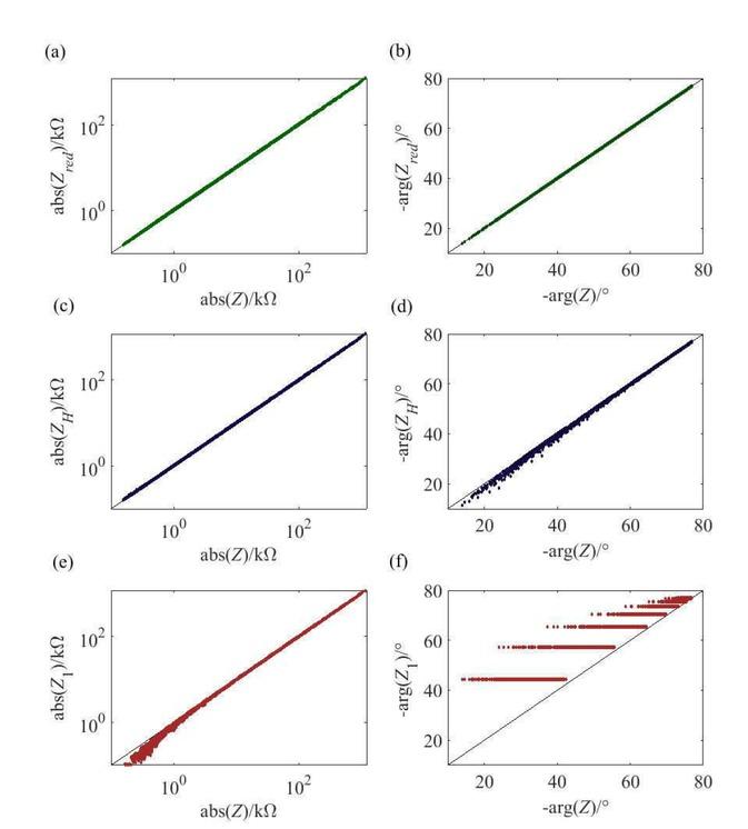
To further test the fidelity of the reduced model, Z_red, and approximate solution, Z_H, let us compare it with the full set of equations for a set of parameters in Table 3 that correspond to different electrode designs with smaller and larger electrodes – w₁, w₂ and w₃ – and thicknesses of stratum corneum, h^SC, and viable skin, h^VS, and frequencies, ν . All permutations of these parameters are considered for a total of 7200 parameter combinations. For the two skin layer thicknesses, we have taken the mean values ± two standard deviations [12]; i.e. 14±6 μm for stratum corneum and 1.2 ± 0.4 mm for viable skin.

Starting with the reduced model in Fig. 5a-b, we see that it captures all the 7200 permutations of the parameters well with respect to the full model – the maximum relative error is 3% and 0.1% for the magnitude and phase respectively. For the approximate solution based on the Hankel transform, Z_H, the picture is slightly different: It agrees well in terms of the predicted magnitude with a maximum relative error of 3% for all parameter combinations, but the error for its predicted phase increases for smaller angles and reaches around 24% for negative phase values of around 20^o.

Fig.5

Verification of the magnitude and the phase of the approximate solutions with the full set of equations for the large parametric study: (a-b) reduced model, Z_red, solved numerically; (c-d) solution, Z_H, from the Hankel transform; (e-f) solution, Z₁, for ℭ≪1.

A closer inspection reveals that the specific parameter combinations for these predicted low negative phase values of around 20^o are as follows: 1 MHz frequency, where the width of the sense, w₁, is typically 3 mm, the width of the inject, w₃, is 3 mm and the spacing between the electrodes, w₂, is 1.2 - 2 mm, whilst h^SC is either 8 or 1.4 μm (but not at the higher thickness of 2 μm) and h^VS is at the lowest thickness of 0.8 mm. The key factors here are the large size of the electrodes (the inject is three times wider than in the base case) and the frequency of 1 MHz, for which ∂Φ/∂z|z=0${{\left. {\partial \Phi }/{\partial z}\; \right|}_{z=0}}$varies significantly across the electrodes, whence the assumption that ∂Φ/∂z|z=0${{\left. {\partial \Phi }/{\partial z}\; \right|}_{z=0}}$is constant for the Hankel solution becomes less accurate. For these conditions, we need to solve the reduced model to maintain low relative errors as compared to the full model. From the point of view of experimental measurements, it should be noted that the standard deviation in the measured phase increases as well when we sweep from 1 kHz to 1 MHz with around 20^o±10^o around 1 MHz [12].

We also see that Z₁ captures the measured magnitude reasonably well at high absolute values of the impedance but grows to a maximum relative error of around 70% at lower values of around 10 kΩ, whereas it only captures the phase close to 1 kHz (values in Fig. 5f close the diagonal) and then fails to describe the measured phase at frequencies larger than 1 kHz with a maximum relative error of around 220%. The latter is due to the fact that Z₁ does not account for the current flow through the viable skin.

At the microscopic level throughout the viable skin, we can determine the point-wise potential distribution by solving the reduced model numerically or take the approximate solution arising from the Hankel transform of the reduced model together with the assumption of constant currents at the electrodes. The latter is given by

(127)Φ(r,z)=c−IHσeffVS×∫0∞cosh[ξ(hVS+z)]sinh(ξhVS)κ(ξ)J0(ξr)dξ.$$\begin{align}& \Phi \left( r,z \right)=\mathfrak{c}-\frac{{{I}_{H}}}{\sigma _{eff}^{VS}}\times \\ & \,\,\,\,\,\,\,\,\int_{0}^{\infty }{\frac{\cosh \left[ \xi \left( {{h}^{VS}}+z \right) \right]}{\sinh \left( \xi {{h}^{VS}} \right)}}\,\kappa \left( \xi \right){{J}_{0}}\left( \xi r \right)d\xi . \\ \end{align}$$

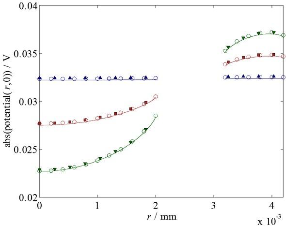
Let us first look at the potential distributions at the electrodes, as depicted in Fig. 6 for the base-case conditions.

Fig.6

The absolute value of the local potential distribution at z=0 m on the base case for the frequencies 1 kHz (▲), 0.328 MHz (_■) and 1 MHz (▼); the reduced numerical model (–) and the Hankel counterpart (o). (N.B.: The verification points have been shifted slightly along r to prevent overlap.)

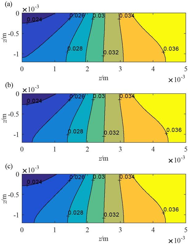
Again, we note the good agreement of the reduced model and approximate solution, Eq. 127, vis-à-vis the complete counterpart with a maximum relative error of around or less than 1%. Throughout the viable skin, the agreement remains good, as can be inferred from the visual comparison of the absolute value of the potential at 1 MHz in Fig. 7.

Fig.7

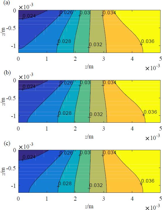
The absolute value of the potential distribution at 1 MHz for the base case in the viable skin: (a) the complete model; (b) the reduced model; and (c) the approximate solution from the Hankel transform.

Finally, we note that we could, although we do not do so here, also calculate and visualize the potential distribution in the stratum corneum by returning to the earlier analysis during which we reduced the stratum corneum to a boundary condition.