
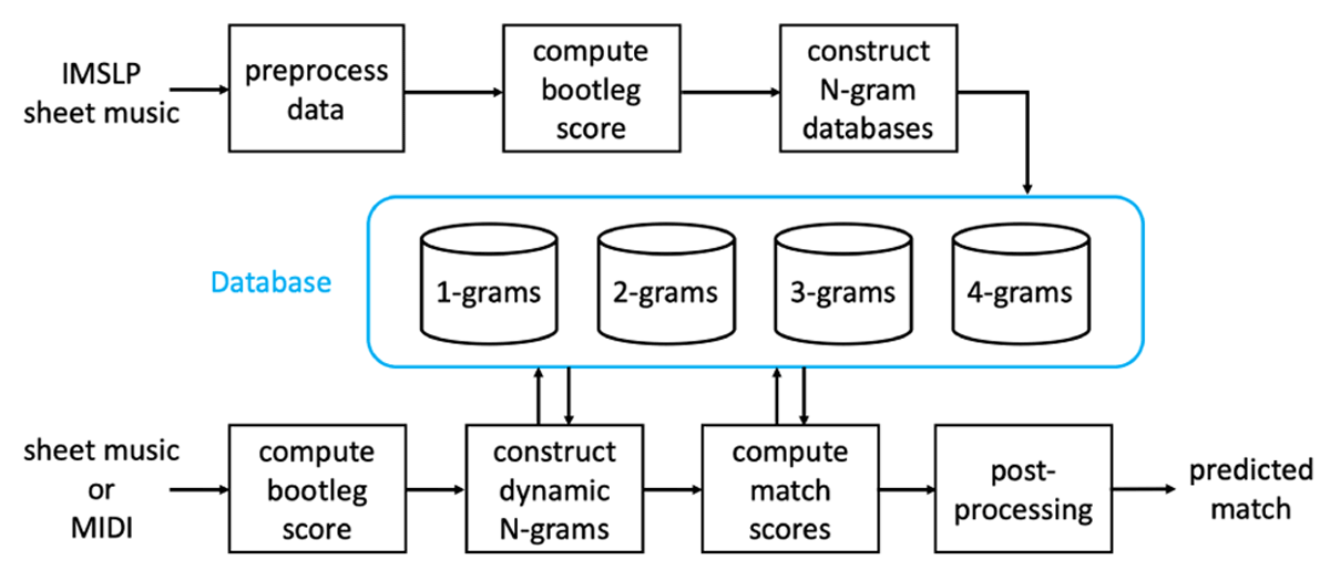
Figure 1
Proposed architecture for large-scale piano sheet music retrieval.
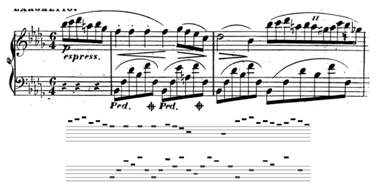
Figure 2
An excerpt of sheet music and its corresponding bootleg score.
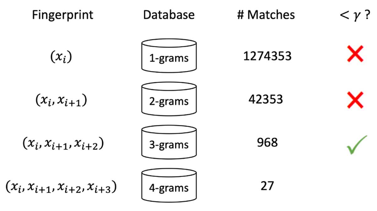
Figure 3
An example of constructing a dynamic N-gram. The length of the N-gram is chosen to balance runtime and retrieval accuracy.
Table 1
Comparing system performance on the camera-based piano sheet music identification task. The first three columns show the mean reciprocal rank on three retrieval tasks at varying levels of specificity. The last two columns show the system runtimes. The 1-gram system was proposed by Tsai (2020) and corresponds to the previous state-of-the-art.
| Retrieval (MRR) | Runtime (s) | ||||
|---|---|---|---|---|---|
| System | Piece | Version | Page | Avg | Sth |
| MAC | .037 | .023 | .026 | 1.17 | .12 |
| SPoC | .003 | .002 | .002 | 1.14 | .09 |
| GeM | .025 | .017 | .017 | 1.18 | .11 |
| R-MAC | .036 | .023 | .024 | 0.96 | .11 |
| 1-gram | .709 | .560 | .620 | 21.5 | 12.5 |
| 2-gram | .845 | .525 | .775 | 2.76 | .36 |
| 3-gram | .808 | .652 | .723 | 1.99 | .21 |
| 4-gram | .755 | .617 | .665 | 1.23 | .13 |
| 5-gram | .608 | .493 | .599 | 1.07 | .08 |
| dynamic | .853 | .692 | .785 | 0.98 | .12 |

Figure 4
Frequency of N-gram fingerprints in the database, where fingerprints have been sorted from most frequent (left) to least frequent (right). Note that both axes are on a log scale.

Figure 5
Effect of database size on system performance for the sheet music identification task. The largest database size corresponds to the full IMSLP piano database.
Table 2
Comparing performance on the sheet music identification task under two conditions: when the exact same printed edition exists in the database (left column) and when only an alternate edition of the same piece exists (right column).
| Piece Retrieval (MRR) | ||
|---|---|---|
| System | Same Version | Alternate Version |
| MAC | .037 | .043 |
| SPoC | .003 | .004 |
| GeM | .025 | .029 |
| R-MAC | .036 | .039 |
| 1-gram | .709 | .659 |
| 2-gram | .845 | .784 |
| 3-gram | .808 | .767 |
| 4-gram | .755 | .722 |
| 5-gram | .688 | .668 |
| dynamic | .853 | .812 |
Table 3
Comparison of system performance on MIDI-sheet image retrieval. Columns indicate the database size (DB), precision (P) and recall (R) and F-measure (F) for passage-level retrieval, mean reciprocal rank (MRR) for file-level retrieval, and average runtime.
| System | DB | P | R | F | MRR | Tavg |
|---|---|---|---|---|---|---|
| Random | 1 | .16 | .16 | .16 | – | 0.0s |
| SharpEye | 1 | .43 | .08 | .13 | – | – |
| PhotoScore | 1 | .64 | .62 | .63 | – | – |
| RetinaNet | 1 | .52 | .26 | .35 | – | 11.7s |
| Dorfer 2018c | 1 | .69 | .28 | .40 | – | 17.5s |
| Faster R-CNN | 1 | .84 | .87 | .85 | – | 49.9s |
| DWD | 1 | .91 | .87 | .89 | – | 213s |
| BS-DTW | 1 | .89 | .89 | .89 | – | 0.90s |
| BS-DTW | 200 | .90 | .87 | .88 | .92 | 10.9s |
| 1-gram | 200 | .58 | .59 | .59 | .69 | 1.28s |
| 2-gram | 200 | .70 | .73 | .71 | .84 | 1.00s |
| 3-gram | 200 | .60 | .72 | .66 | .79 | 1.00s |
| 4-gram | 200 | .41 | .57 | .48 | .63 | 1.00s |
| 5-gram | 200 | .36 | .49 | .42 | .53 | 1.00s |
| dynamic | 200 | .74 | .77 | .75 | .86 | 0.98s |
| BS-DTW | 2k | .89 | .83 | .86 | .88 | 167s |
| 1-gram | 2k | .48 | .51 | .49 | .59 | 2.28s |
| 2-gram | 2k | .63 | .69 | .66 | .78 | 1.10s |
| 3-gram | 2k | .49 | .63 | .55 | .69 | 1.09s |
| 4-gram | 2k | .39 | .55 | .46 | .60 | 1.04s |
| 5-gram | 2k | .35 | .47 | .40 | .51 | 1.05s |
| dynamic | 2k | .66 | .72 | .69 | .80 | .98s |
| BS-DTW | 10k | .83 | .77 | .80 | .83 | 458s |
| 1-gram | 10k | .28 | .34 | .31 | .43 | 6.78s |
| 2-gram | 10k | .43 | .58 | .49 | .68 | 1.45s |
| 3-gram | 10k | .40 | .53 | .46 | .56 | 1.10s |
| 4-gram | 10k | .34 | .48 | .40 | .50 | 1.04s |
| 5-gram | 10k | .28 | .42 | .34 | .46 | 1.00s |
| dynamic | 10k | .55 | .66 | .60 | .73 | .99s |
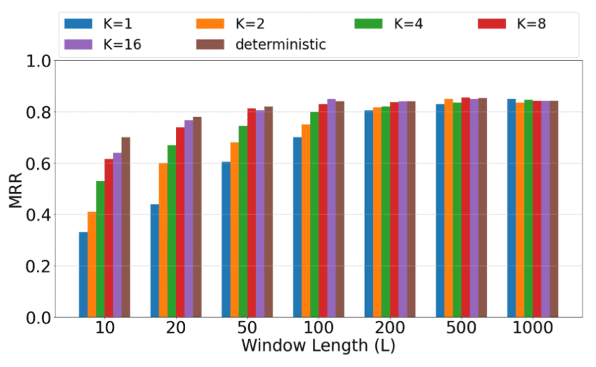
Figure 6
Comparing different strategies for handling repeats and jumps in MIDI-sheet image retrieval. The MIDI query is broken up into fragments of length L, either through deterministic shingling or a fixed number (K) of randomly sampled windows.