
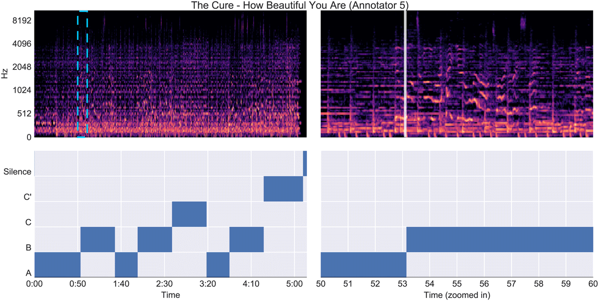
Figure 1
Example of a flat structure annotation (track 10 from SALAMI). The left side displays the full track; a zoomed-in version of a segment boundary (marked with a dashed light blue rectangle on the left) is shown on the right. On top, log-mel power spectrograms of the audio signal are displayed, while at the bottom the annotations are plotted.

Figure 2
SSM prototype of track 10 from SALAMI. Blocks contain homogeneous segments, diagonals represent repetitions (except the main one), and dashed-lines depict the reference annotation.
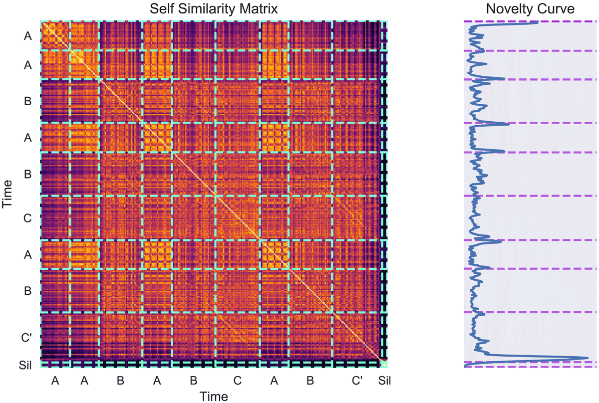
Figure 3
Self similarity matrix (left) and its associated novelty curve (right) of track 10 from SALAMI. Brighter colors in the SSM indicate a greater degree of similarity. Dashed lines mark segment boundaries identified by annotator 5.
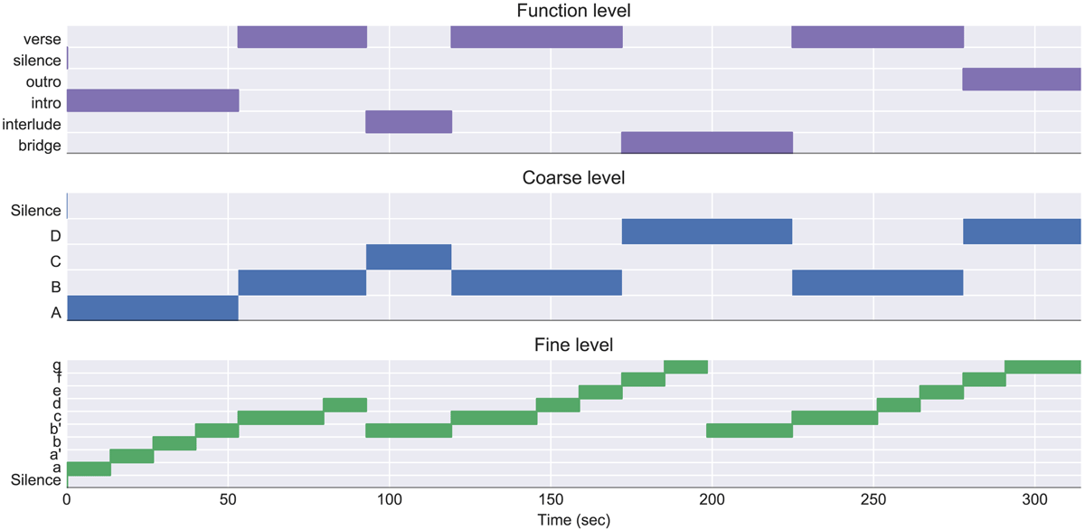
Figure 4
Example of a hierarchical structure annotation from annotator 4 of track 10 in SALAMI. The functional level is plotted on top. In the middle, the coarse level is shown, with notable differences from those segmentations plotted in Figure 1 due to annotators disagreements. In the bottom, the fine level is displayed.
Table 1
Best performing evaluation metrics (percentages) for the MSA task in MIREX for the years 2012 to 2017. *: Smaller subset of SALAMI; †: 2015 submission by Grill and Schlüter (2015a); ‡: 2012 submission by Serrà et al. (2014); §: 2014 submission by Ullrich et al. (2014).
| Dataset | |||
| MIREX 2009 | 56.42 ± 17.04† | 70.35 ± 14.87† | 65.28 ± 15.11‡ |
| MIREX 2010 (1) | 69.70 ± 13.59† | 79.34 ± 9.43† | – |
| MIREX 2010 (2) | 52.37 ± 17.54† | 73.80 ± 11.68§ | 68.83 ± 11.91‡ |
| SALAMI* | 54.09 ± 18.50† | 68.94 ± 17.51§ | 58.09 ± 15.77‡ |