
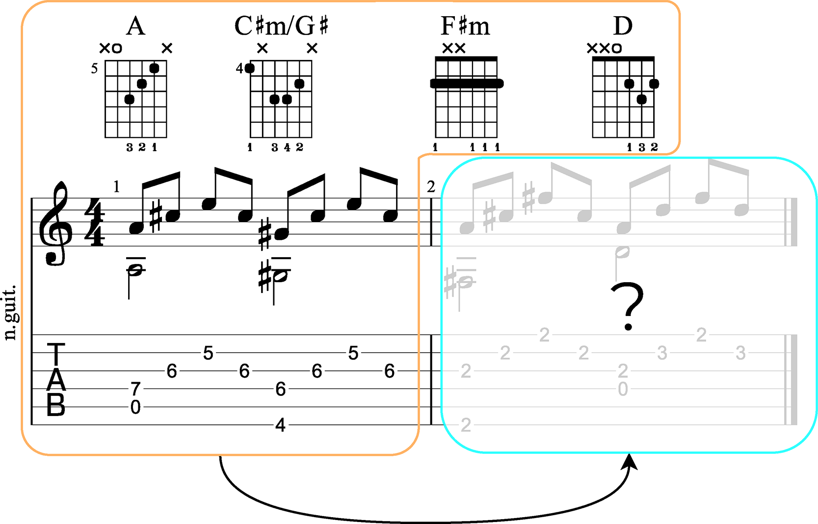
Figure 1
Excerpt of a rhythm guitar tablature showing a summary of the studied task: a tablature excerpt is taken as input and, given the underlying chord progression, a tablature continuation is suggested.
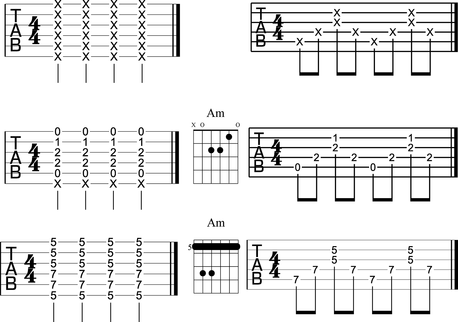
Figure 2
Two picking patterns (top) and the corresponding tablatures for two Am chord diagrams.
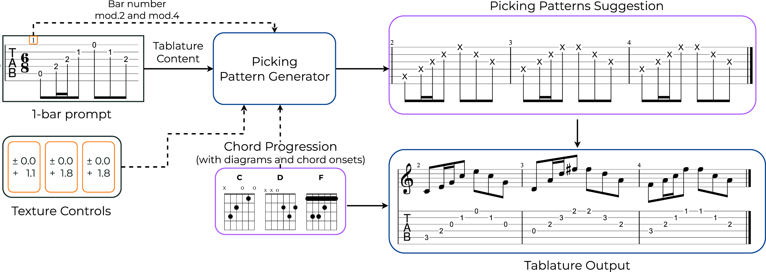
Figure 3
Overview of the picking pattern generation pipeline. The final tablature is obtained by combining the chord diagrams with the generated picking patterns. The texture controls convey the expected distance of bars 2 to 4 (left to right) with respect to the first bar for horizontal (top values) and vertical (bottom values) texture values.
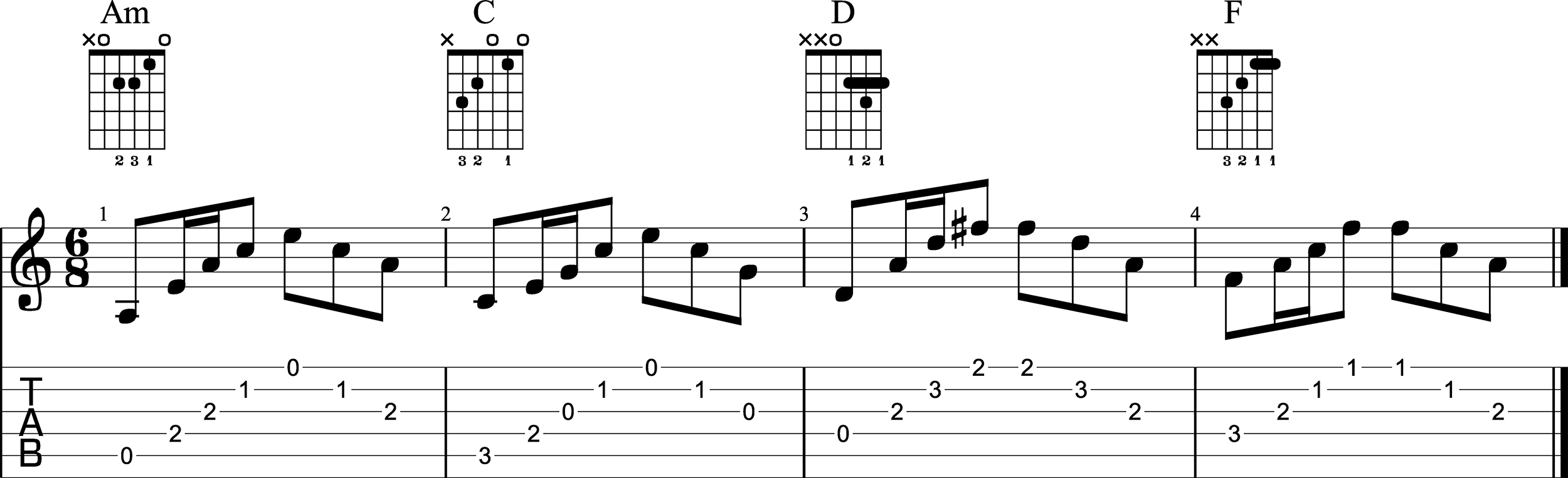
Figure 4
Example of a rhythm guitar part tablature including four chord regions with similar/uniform texture. Excerpt from The House of the Rising Sun by The Animals.
Table 1
Tokens in the vocabulary. Note: token:n‑m means that the value for token can be any integer between n and m inclusive.
| Type | Tokens | Voc. Size |
|---|---|---|
| Metadata | <start>, <end>, <bar>, <PAD> | 4 |
| Note | string:1‑6, rest | 7 |
| Onset | onset:0‑47 | 48 |
| Duration | duration:1‑96 | 96 |
| Total | 155 |
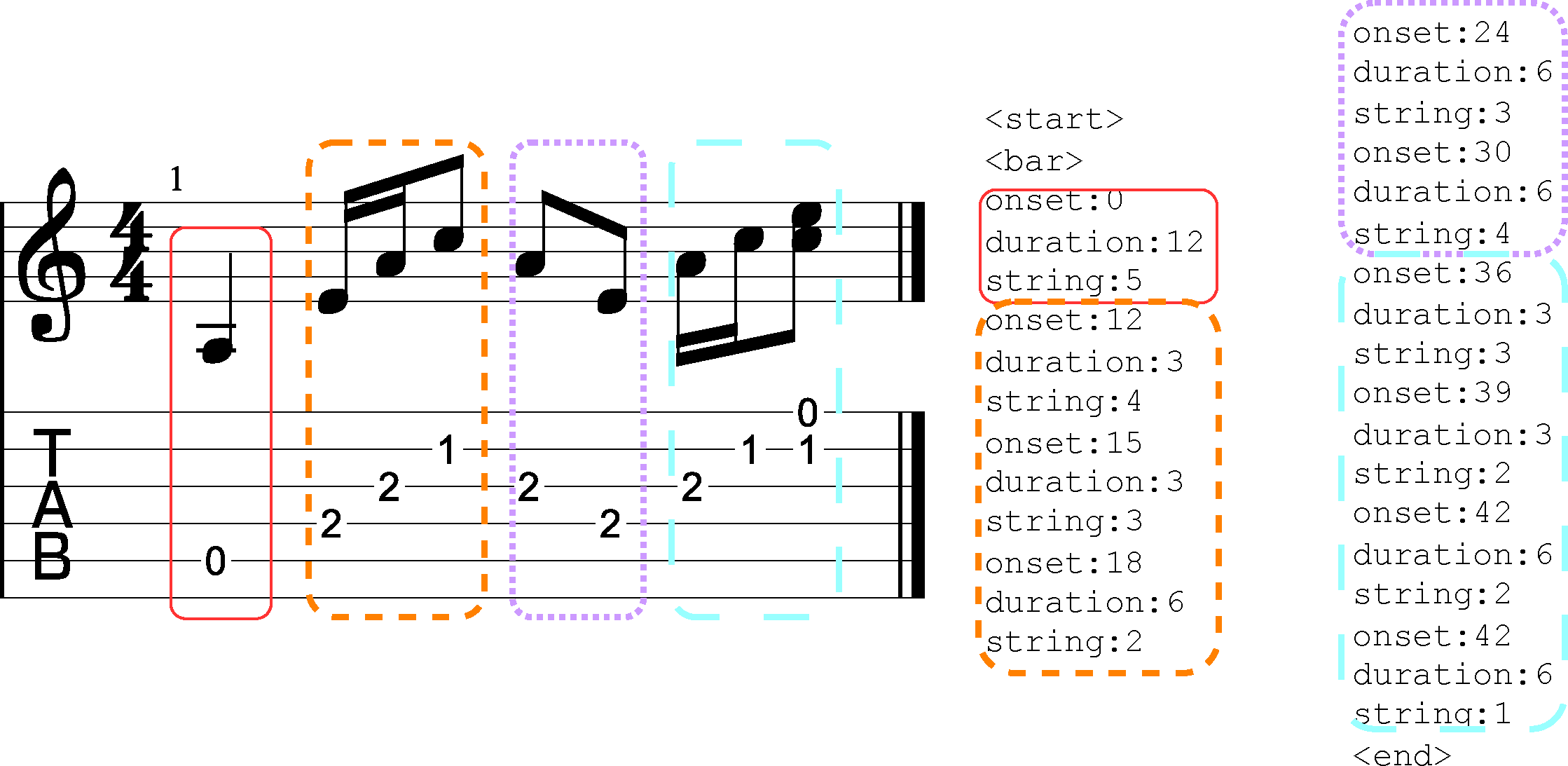
Figure 5
Example of the tokens obtained from a single bar tablature excerpt.
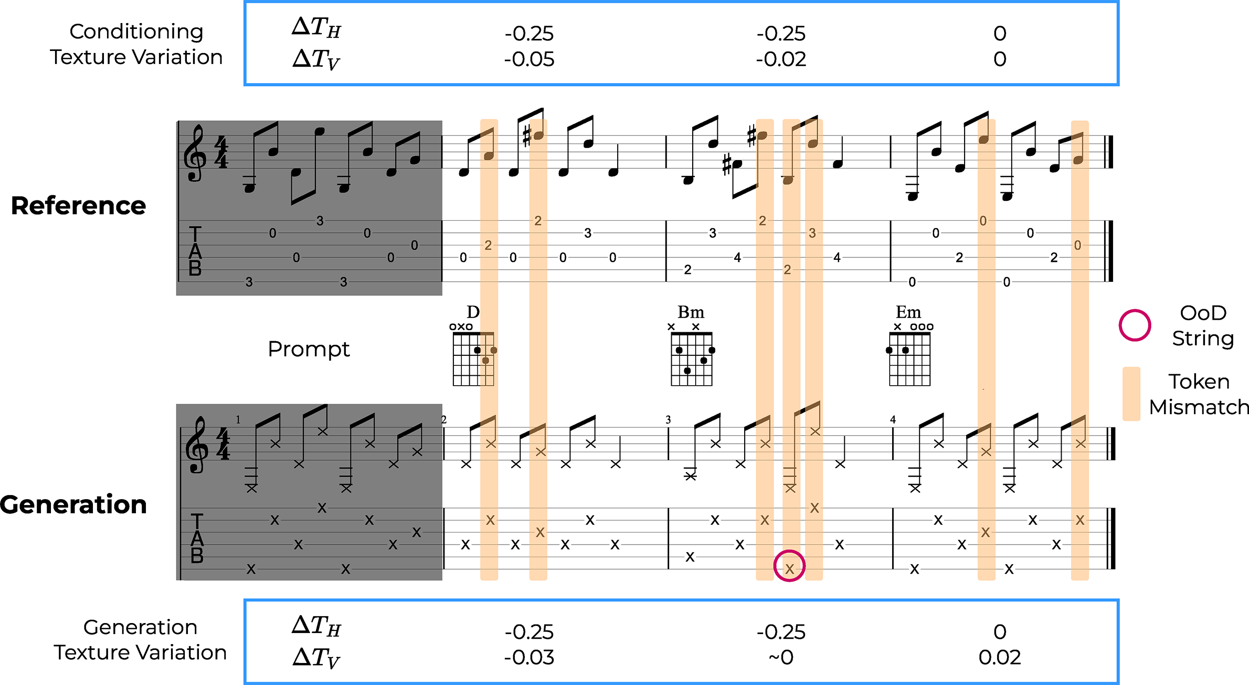
Figure 6
Comparison between the generated picking pattern (bottom) and the reference tablature (top): the edit distance is 7, or 0.1 after normalization; the ratio of OoD notes is 0.05; and the texture distance, calculated using the Manhattan distance, is 0.06.
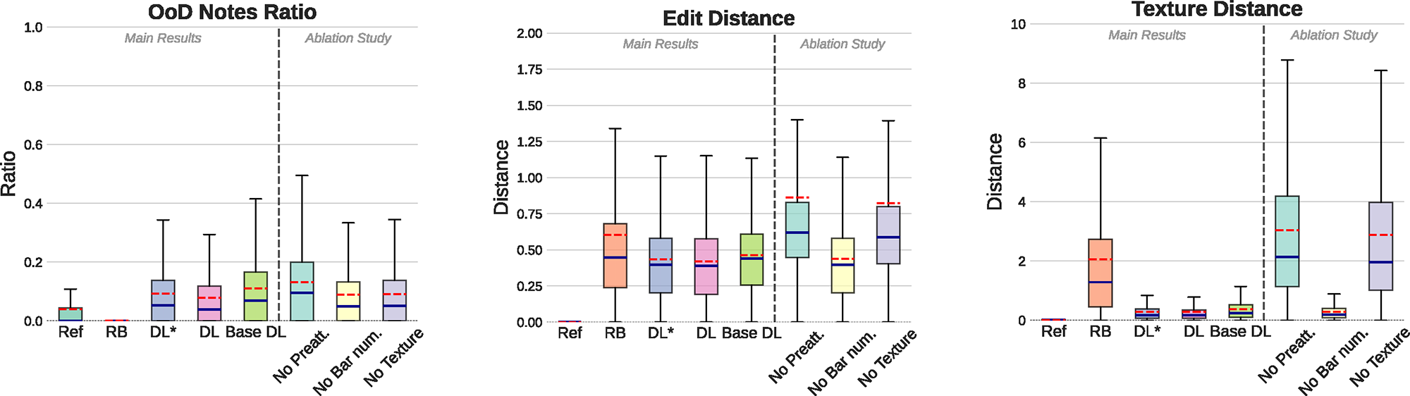
Figure 7
Box plot distributions of the results from several model configurations; the red dashed lines show the average of each distribution. The outliers are not shown to increase readability. ‘Ref’ stands for the ground‑truth data, RB stands for the rule‑based model. DL stands for the complete deep learning model, DL* is the same model without a diagram loss during the second training phase, and ‘Base DL’ is the DL model before conducting the second training phase. We used Wilcoxon signed‑rank tests to verify statistical significance, with a Bonferroni‑corrected significance threshold . All pairwise differences are highly significant (), except for four of them, which are detailed in Section 7. The rightmost part of each subplot shows the performance of the DL model with ablated parts, such as no preattention, no bar number information, or no texture controls. All distributions are significantly different (p ) from the complete DL model.
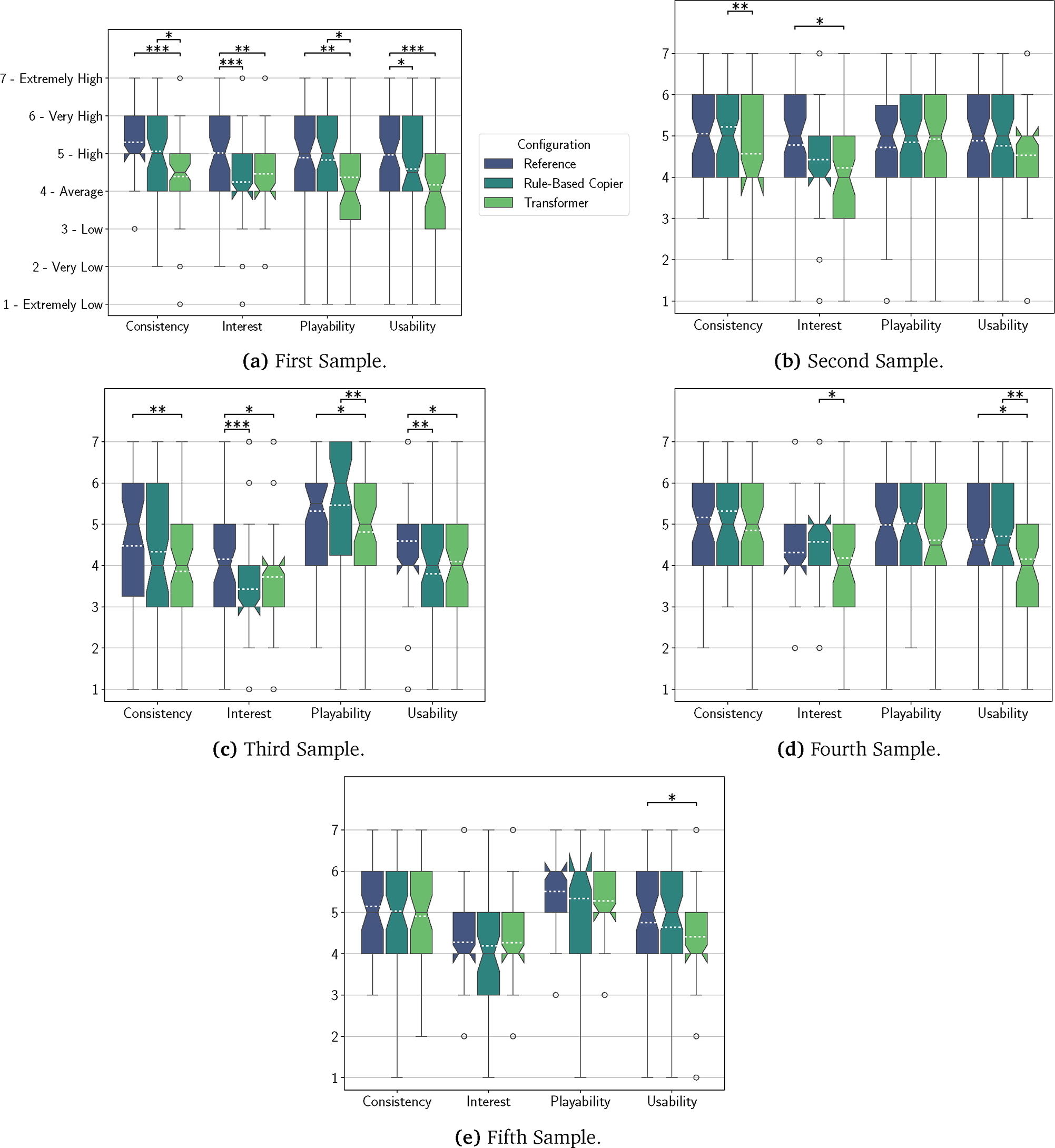
Figure 8
Boxplots of the participants’ answers for each question and each sample. The boxes indicates the distributions’ quartiles, while the whiskers describe all others samples that are not considered outliers (denoted by empty circles). Notches around the median show the confidence interval, and the dotted lines represent the average answer values. Brackets indicate statistical significance in pairwise Wilcoxon signed‑rank tests (non‑normality of the data was checked beforehand) using a Bonferroni‑adjusted level of : *, **,***.
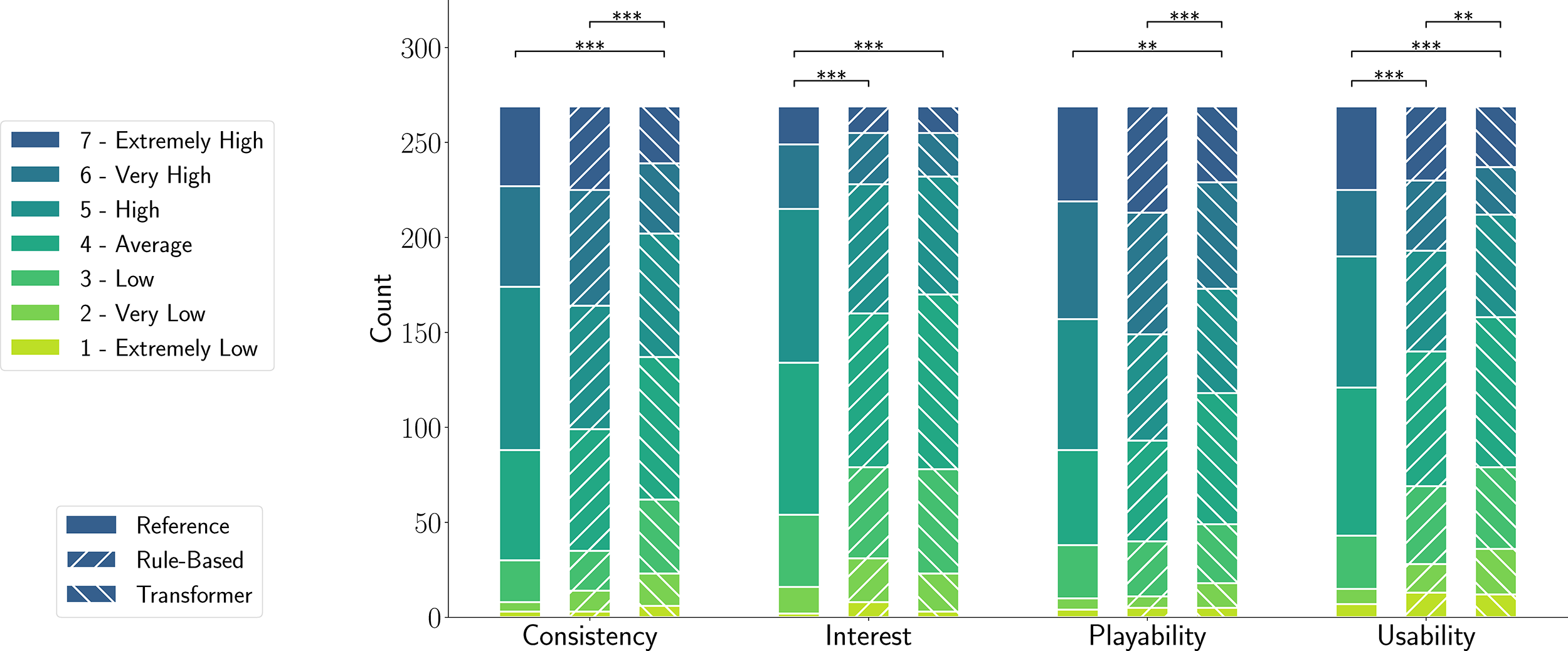
Figure 9
Cumulated answers on all five questions for each configuration. Brackets indicate statistical significance in pairwise Wilcoxon signed‑rank tests (non‑normality of the data was checked beforehand) using a Bonferroni‑adjusted level of : *, **,***.
Table 2
Results of the linear mixed‑effects model analysis. The intercept is the base answer value observed, while the models and samples are compared to the reference or the first sample, respectively.
| Variable | Coeff. | Std. Err. | ||
|---|---|---|---|---|
| Intercept | 5.692 | 0.382 | 14.917 | |
| Model: Rule‑Based | −0.156 | 0.056 | −2.814 | |
| Model: Transformer | −0.402 | 0.056 | −7.225 | |
| Sample 2 | 0.032 | 0.072 | 0.448 | |
| Sample 3 | −0.361 | 0.072 | −5.035 | |
| Sample 4 | 0.026 | 0.072 | 0.358 | |
| Sample 5 | 0.143 | 0.072 | 1.978 | |
| Participant Variance | 0.503 | 0.094 |