
Table 1
The 10 protochords of the GCT model, considering genealogical and alphanumeric notations. The symbol * stands for a generic root.
| Genera | Genealogical notation | Alphanumeric notation |
|---|---|---|
| Z | Z0 | *M7 |
| Y | Y0 | *7 |
| X | X0 | *(♭5)7 |
| W | W0 | *(♯5)7 |
| V | V0 | * |
| z | z0 | *m7 |
| y | y0 | |
| x | x0 | *°7 |
| w | w0 | *m(M7) |
| v | v0 | *m |
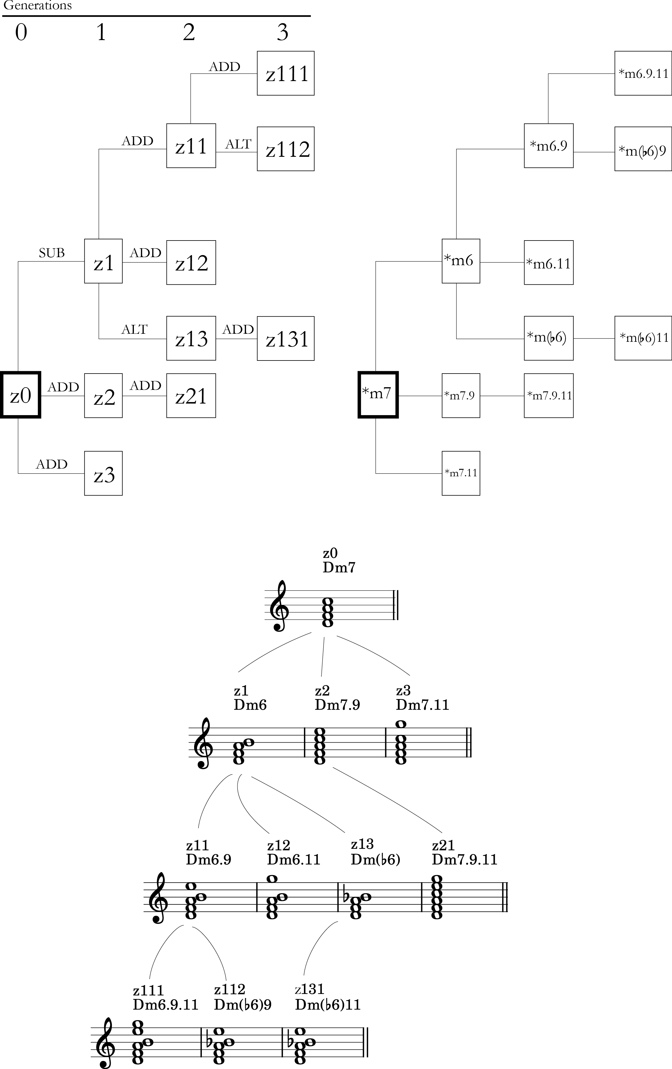
Figure 1
Genus of protochord z0 depicted in three notations: genealogical (top left), chord‑label (top right – using the symbol * as a generic root.), and musical (below – using ‘D’ as the reference root).
Table 2
Distribution of CTs across the 10 genera (shown in the rows), considering a total of six possible generations (shown in the columns). The total number of variations for each genera across all the generations is displayed in the last column; the total number of variations in each generation across all genera is displayed in the last row.
| Genera | 0 | 1 | 2 | 3 | 4 | 5 | 6 | Total |
|---|---|---|---|---|---|---|---|---|
| Z | 1 | 5 | 7 | 3 | – | – | – | 16 |
| Y | 1 | 4 | 9 | 14 | 16 | 13 | 2 | 59 |
| X | 1 | 3 | 5 | 6 | 4 | – | – | 19 |
| W | 1 | 2 | 3 | 3 | 1 | – | – | 10 |
| V | 1 | 4 | 5 | 2 | – | – | – | 12 |
| z | 1 | 3 | 4 | 3 | – | – | – | 11 |
| y | 1 | 3 | 3 | 1 | – | – | – | 8 |
| x | 1 | 4 | 6 | 3 | 1 | – | – | 15 |
| w | 1 | 2 | 1 | – | – | – | – | 4 |
| v | 1 | 3 | 3 | 1 | – | – | – | 8 |
| Total | 10 | 33 | 46 | 36 | 22 | 13 | 2 | 161 |
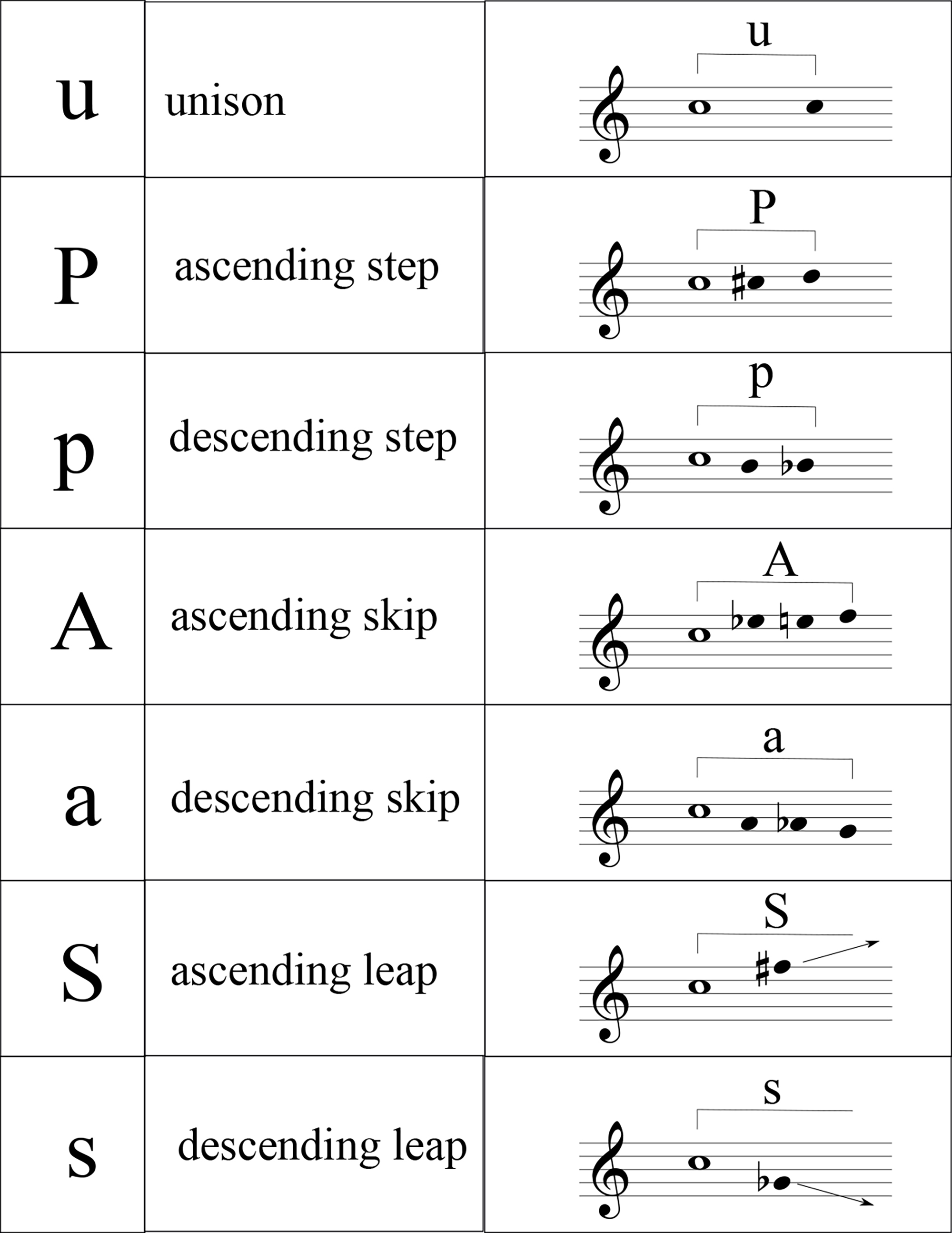
Figure 2
Alphabet of c‑letters, their description, and an illustration of the distances encoded by each letter, starting from a C note.
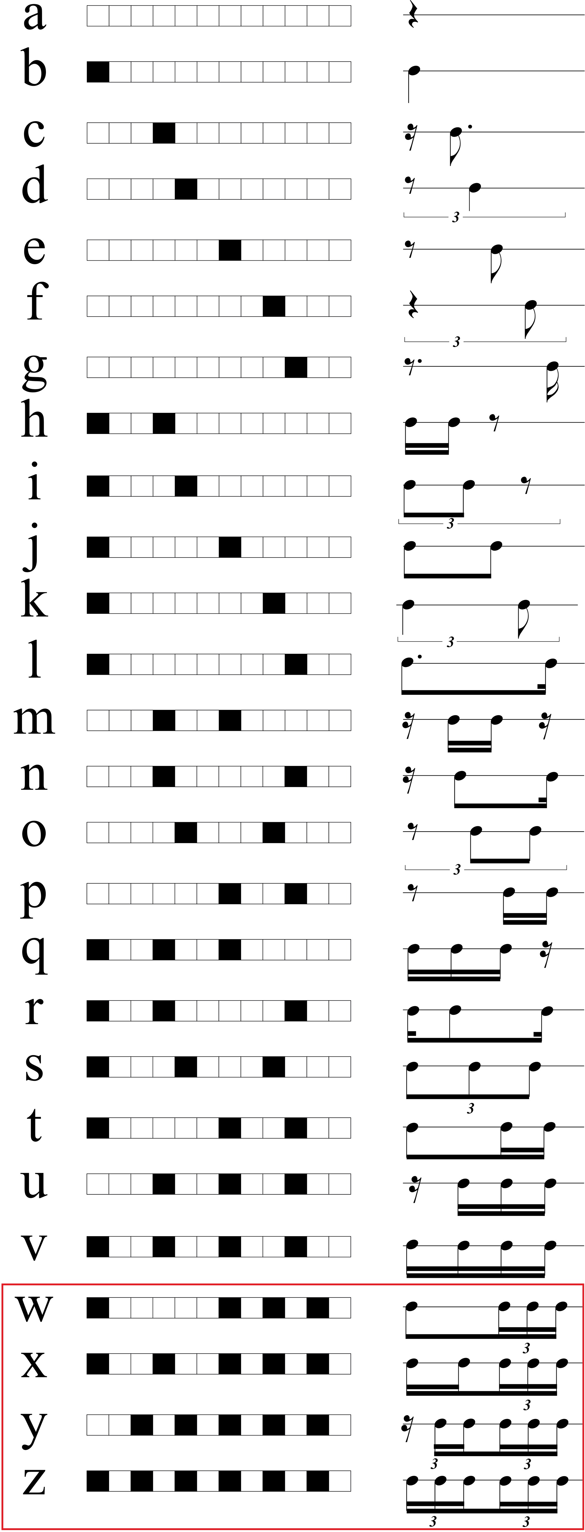
Figure 3
Alphabet of r‑letters.
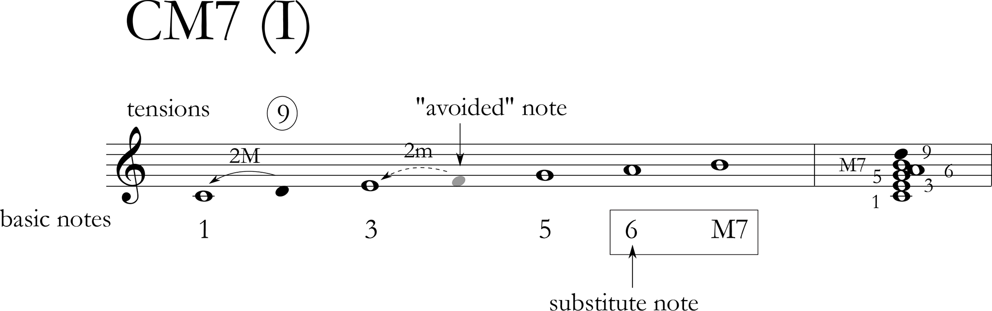
Figure 4
Structure of the CM7 scale (I in C major) and identification of its structural notes.
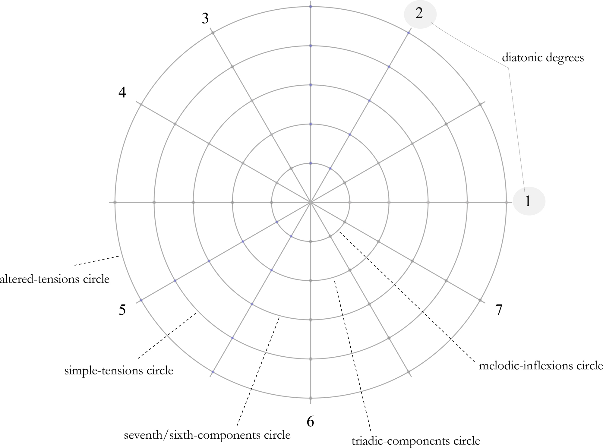
Figure 5
Basic scheme of the NF web in major mode.
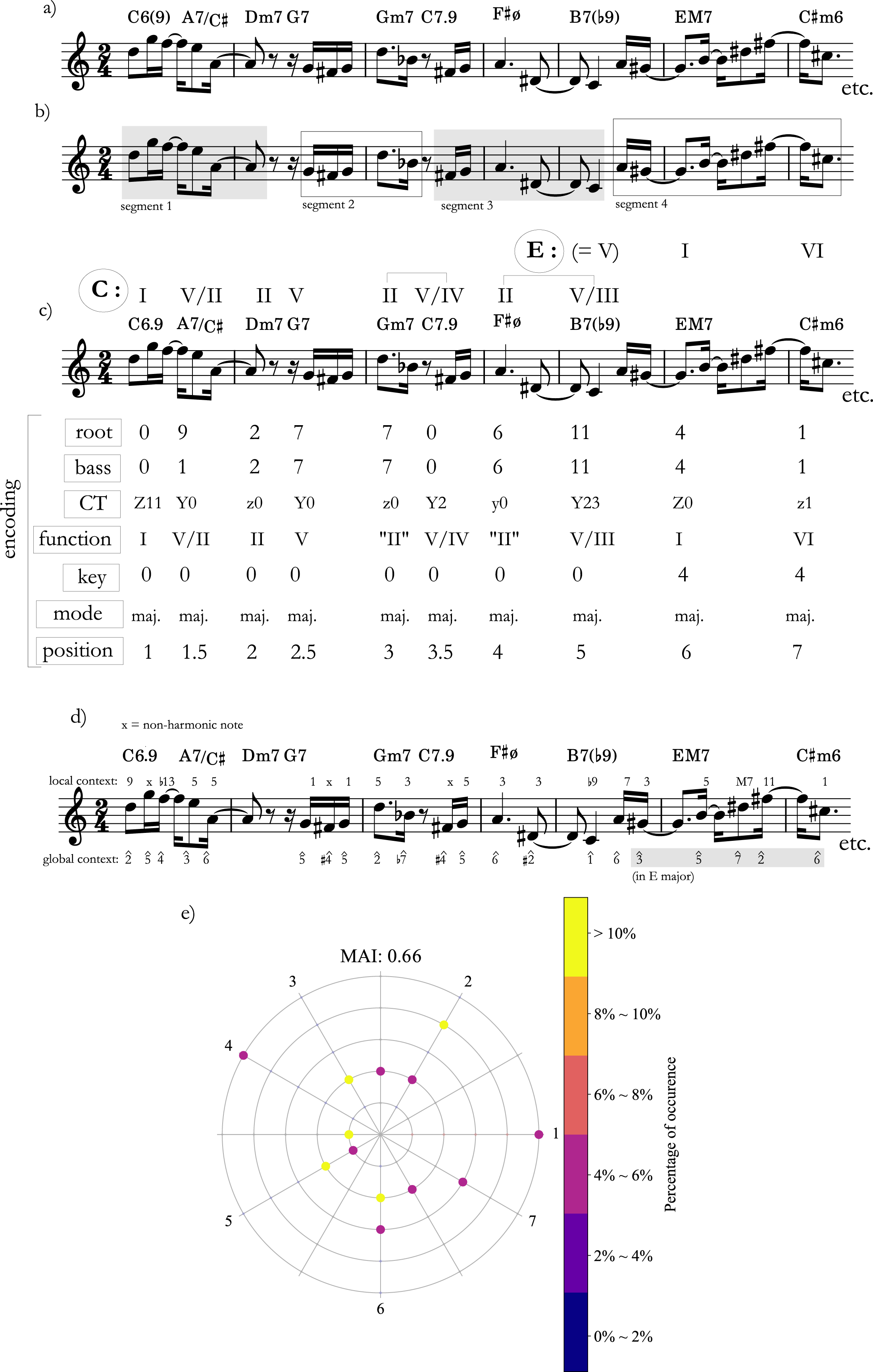
Figure 6
Example of the analytical process: a) excerpt being analyzed; b) segmentation of the melody; c) harmonic analysis; d) relation between melody and harmony; and e) NF web of this excerpt. For more details on the notation, see Section 3.
Table 3
Correspondence between the abbreviated corpus names (column ‘corpus_id’ within all the files of the dataset) and the artistic names of the respective composers.
| corpus_id | Composer’s artistic name |
|---|---|
| JOBIM | Tom Jobim |
| LINS | Ivan Lins |
| CHICO | Chico Buarque |
| EDU | Edu Lobo |
| CAETANO | Caetano Veloso |
| DJAVAN | Djavan |
| BOSCO | João Bosco |
| MILTON | Milton Nascimento |
| GIL | Gilberto Gil |
| RITA | Rita Lee |
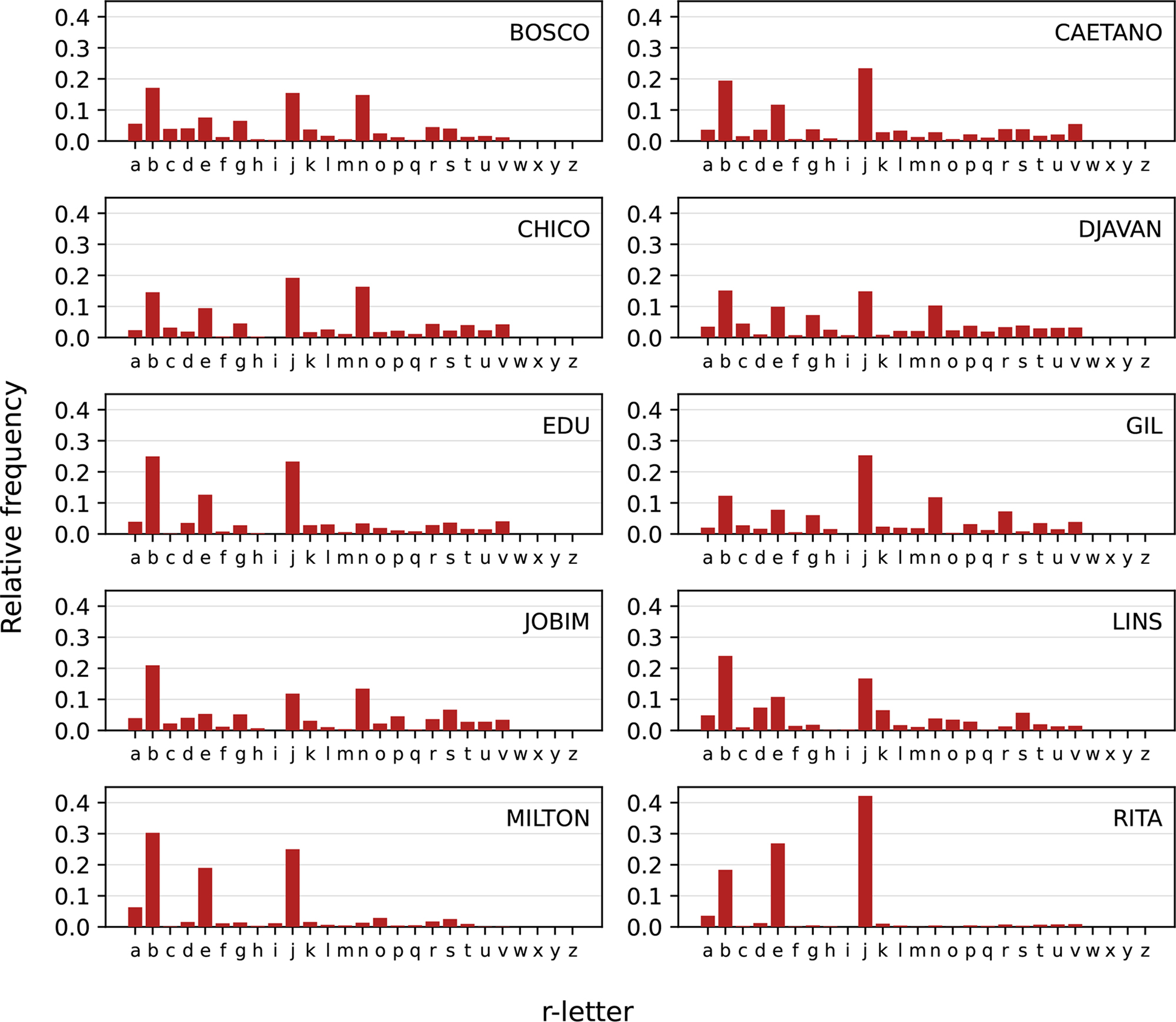
Figure 7
Bar chart showing the proportion of each r‑letter in each examined corpora.
Table 4
Metric profile by analyzed corpus, in percentage. The columns contain only the attack points present in the corpora. Percentages in bold correspond to the most prominent attack point on each corpus.
| 1 | 4 | 5 | 7 | 9 | 10 | |
|---|---|---|---|---|---|---|
| Bosco | 31.5 | 17.0 | 6.7 | 18.1 | 7.1 | 20.2 |
| Caetano | 37.6 | 10.9 | 4.7 | 27.9 | 4.5 | 14.4 |
| Chico | 29.6 | 18.0 | 3.2 | 23.8 | 3.3 | 22.1 |
| Djavan | 29.3 | 17.6 | 4.5 | 23.7 | 4.4 | 20.5 |
| Edu | 40.7 | 8.3 | 5.5 | 27.6 | 5.5 | 12.4 |
| Gil | 32.3 | 17.1 | 1.5 | 25.8 | 2.2 | 21.0 |
| Jobim | 31.0 | 15.3 | 7.4 | 17.8 | 7.5 | 20.9 |
| Lins | 38.2 | 6.7 | 10.7 | 23.2 | 10.9 | 10.4 |
| Milton | 46.5 | 3.5 | 5.9 | 33.4 | 5.8 | 4.9 |
| Rita | 43.5 | 2.6 | 1.1 | 48.2 | 1.1 | 3.4 |
Table 5
Distribution of countermetric r‑letters by corpus, in percentage. The last column shows the total occurrence of these r‑letters for each composer. The most prominent countermetric r‑letter in each corpus is highlighted in bold.
| c | e | g | m | n | p | u | Total | |
|---|---|---|---|---|---|---|---|---|
| Bosco | 3.9 | 7.6 | 6.5 | 0.6 | 14.8 | 1.2 | 1.6 | 36.2 |
| Caetano | 1.6 | 11.7 | 3.8 | 1.3 | 2.8 | 2.1 | 2.1 | 25.4 |
| Chico | 3.2 | 9.5 | 4.5 | 1.1 | 16.3 | 2.2 | 2.3 | 39.2 |
| Djavan | 4.5 | 9.9 | 7.2 | 2.1 | 10.3 | 3.8 | 3.1 | 40.9 |
| Edu | 0.2 | 12.6 | 2.8 | 0.6 | 3.4 | 1.1 | 1.5 | 22.3 |
| Gil | 2.8 | 7.8 | 6.1 | 1.9 | 11.8 | 3.2 | 1.5 | 35.0 |
| Jobim | 2.2 | 5.3 | 5.2 | 0.4 | 13.4 | 4.5 | 2.8 | 33.9 |
| Lins | 1.0 | 10.8 | 1.8 | 1.1 | 3.9 | 2.8 | 1.3 | 22.8 |
| Milton | 0.2 | 19.0 | 1.4 | 0.5 | 1.4 | 0.5 | 0.1 | 23.1 |
| Rita | 0.3 | 26.9 | 0.5 | 0.1 | 0.5 | 0.5 | 0.8 | 29.6 |
Table 6
Statistics related to melodic contour, melodic rhythm, and the relationship between melody and harmony. The columns represent, respectively: length of the most common c‑ and r‑word, CIEI, CMI, and MAI indexes.
| Word length | CIEI | CMI | MAI | |
|---|---|---|---|---|
| Bosco | 8 | 0.856 | 0.559 | 0.704 |
| Caetano | 7 | 0.873 | 0.463 | 0.721 |
| Chico | 6 | 0.887 | 0.564 | 0.704 |
| Djavan | 6 | 0.863 | 0.558 | 0.643 |
| Edu | 8 | 0.867 | 0.463 | 0.623 |
| Gil | 8 | 0.880 | 0.552 | 0.714 |
| Jobim | 6 | 0.888 | 0.531 | 0.582 |
| Lins | 7 | 0.867 | 0.446 | 0.649 |
| Milton | 6 | 0.898 | 0.388 | 0.684 |
| Rita | 5 | 0.886 | 0.429 | 0.741 |
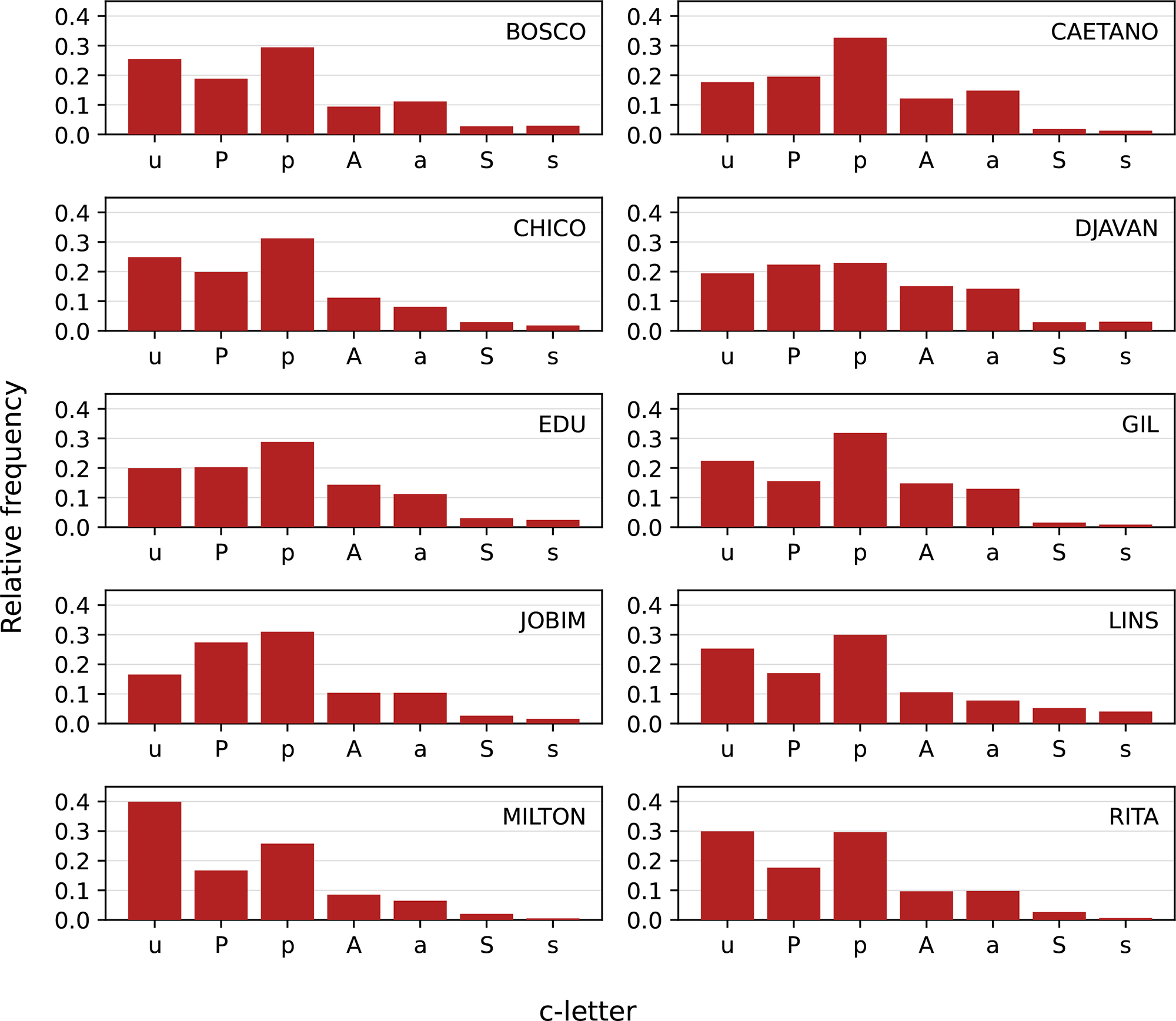
Figure 8
Bar chart showing the proportion of each c‑letter in each examined corpora.
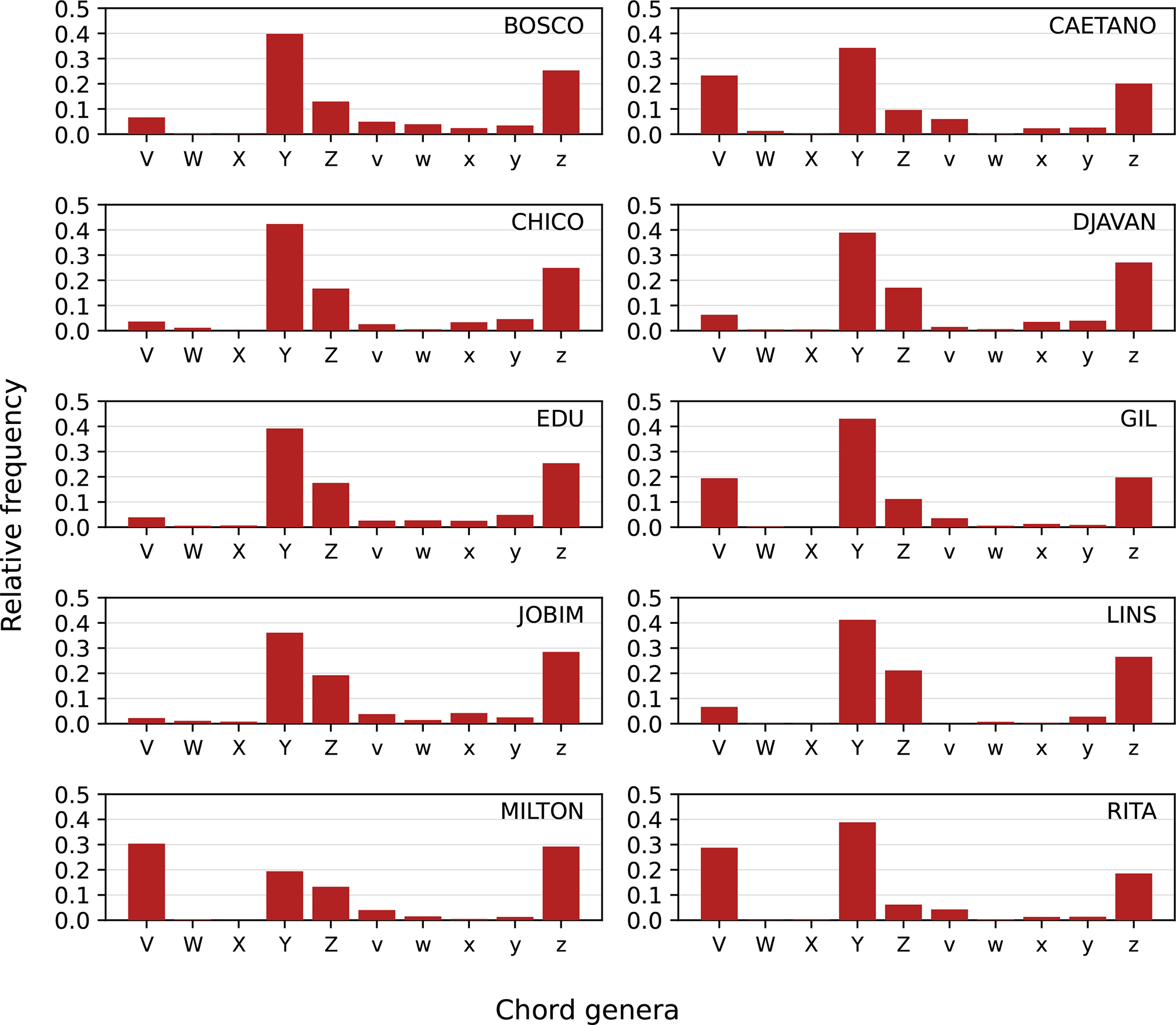
Figure 9
Bar chart showing the proportion of each chord genera in each examined corpora.
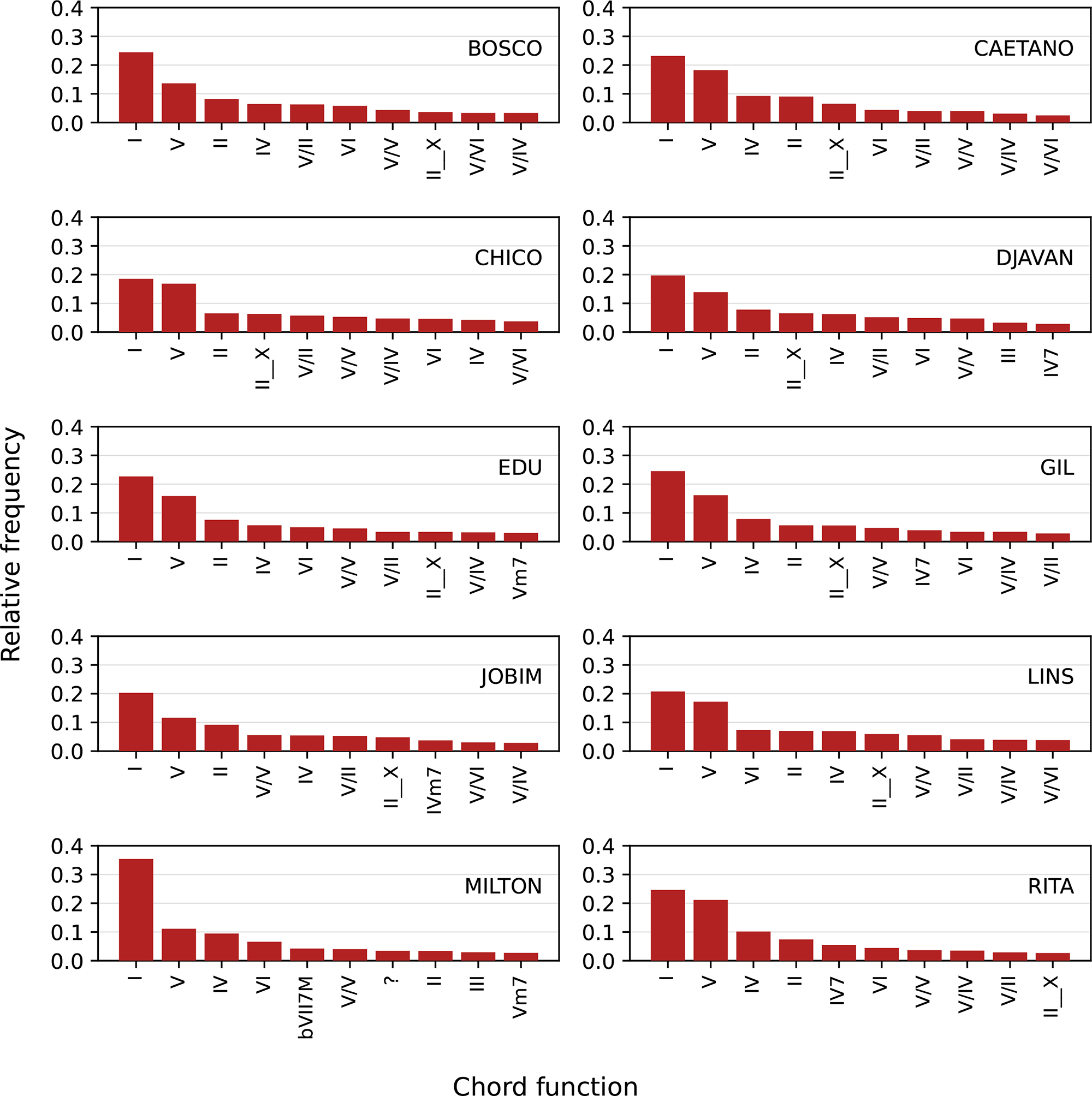
Figure 10
Bar chart showing the proportion of the most common chord functions in each examined corpora.
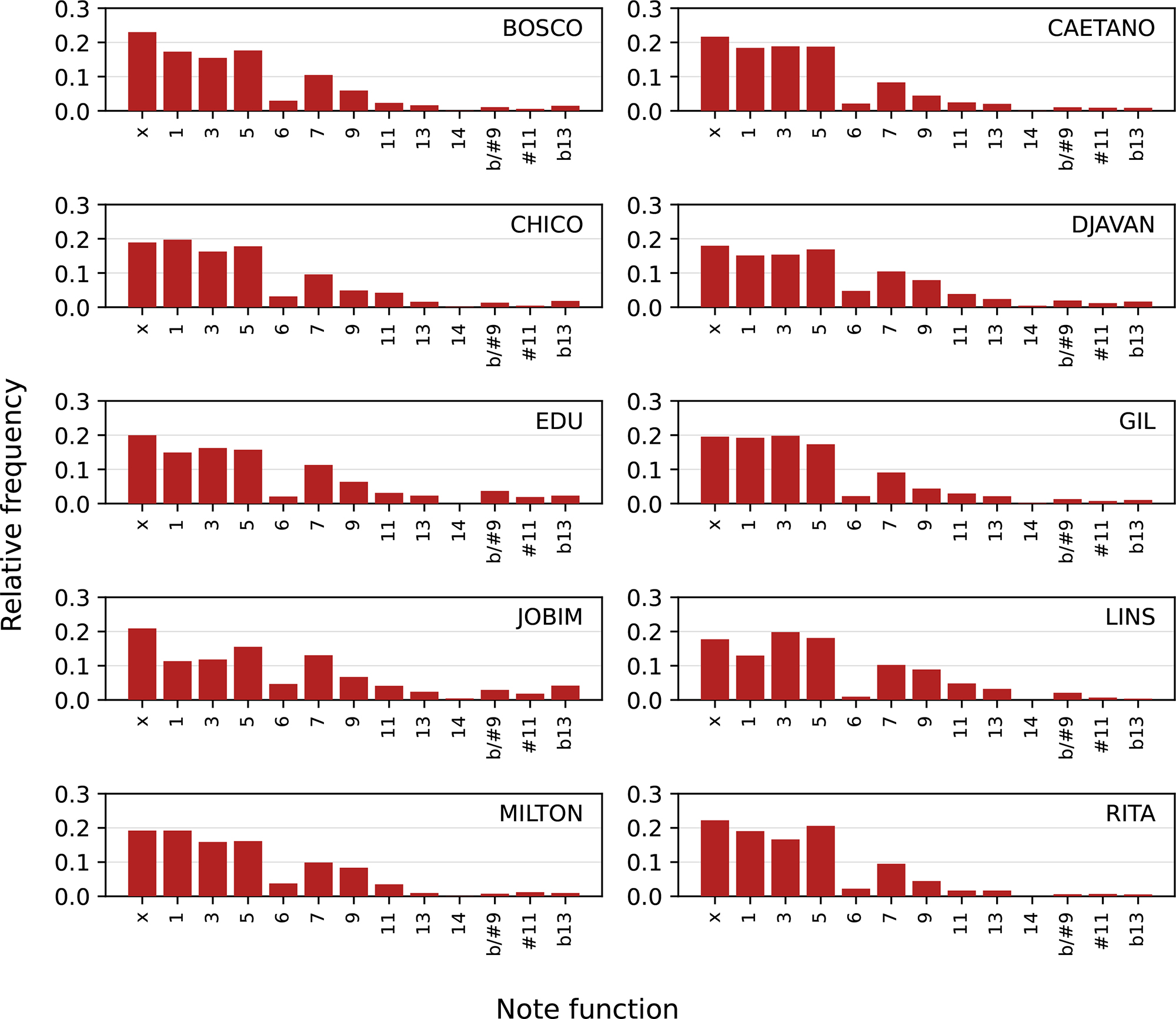
Figure 11
Bar chart showing the proportion of each note function in each examined corpora.
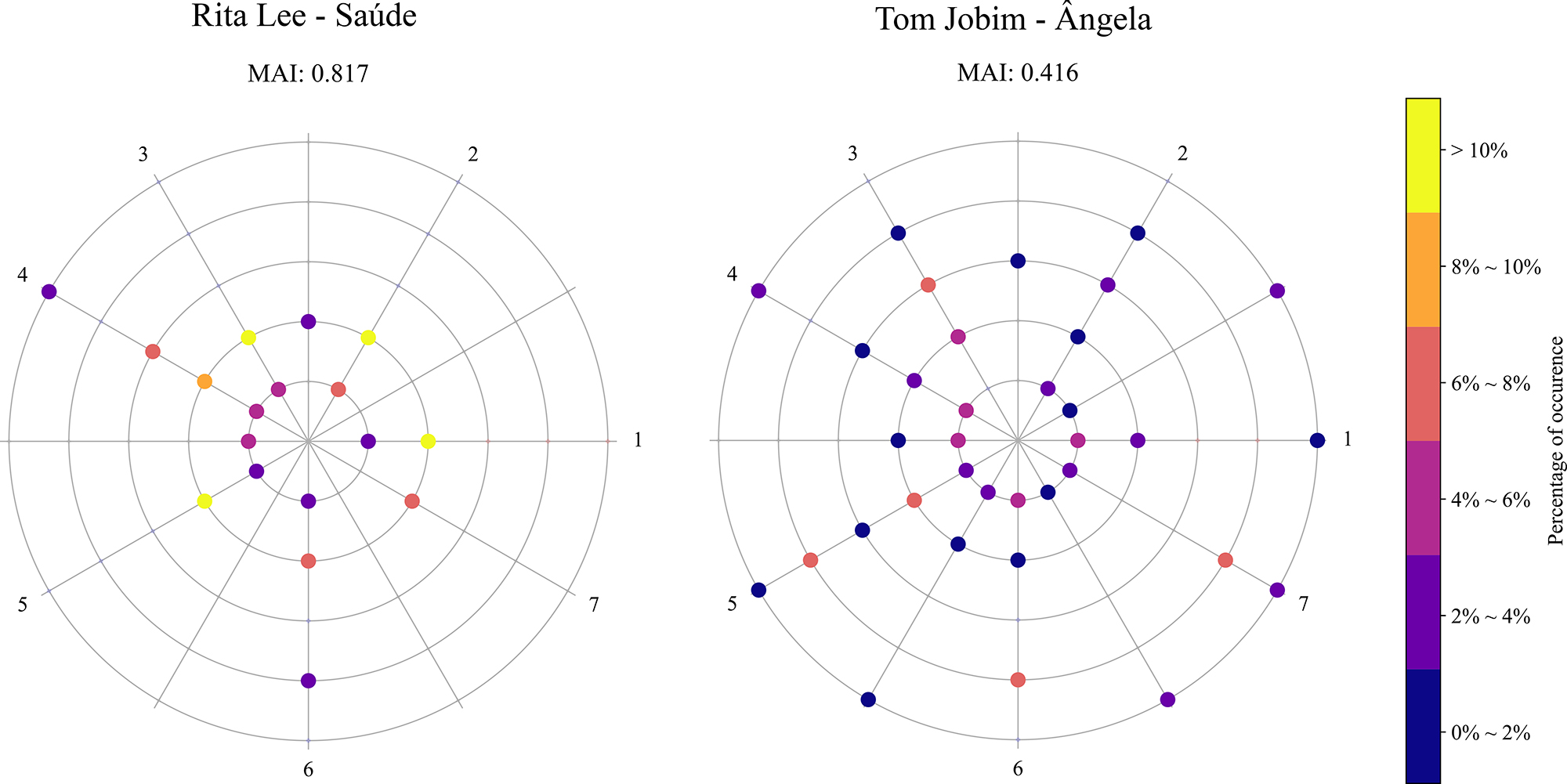
Figure 12
NF web of two pieces: Saúde, by Rita Lee (left panel), and Angela, by Tom Jobim (right panel). Their respective melodic anchoring indices are displayed above the webs.
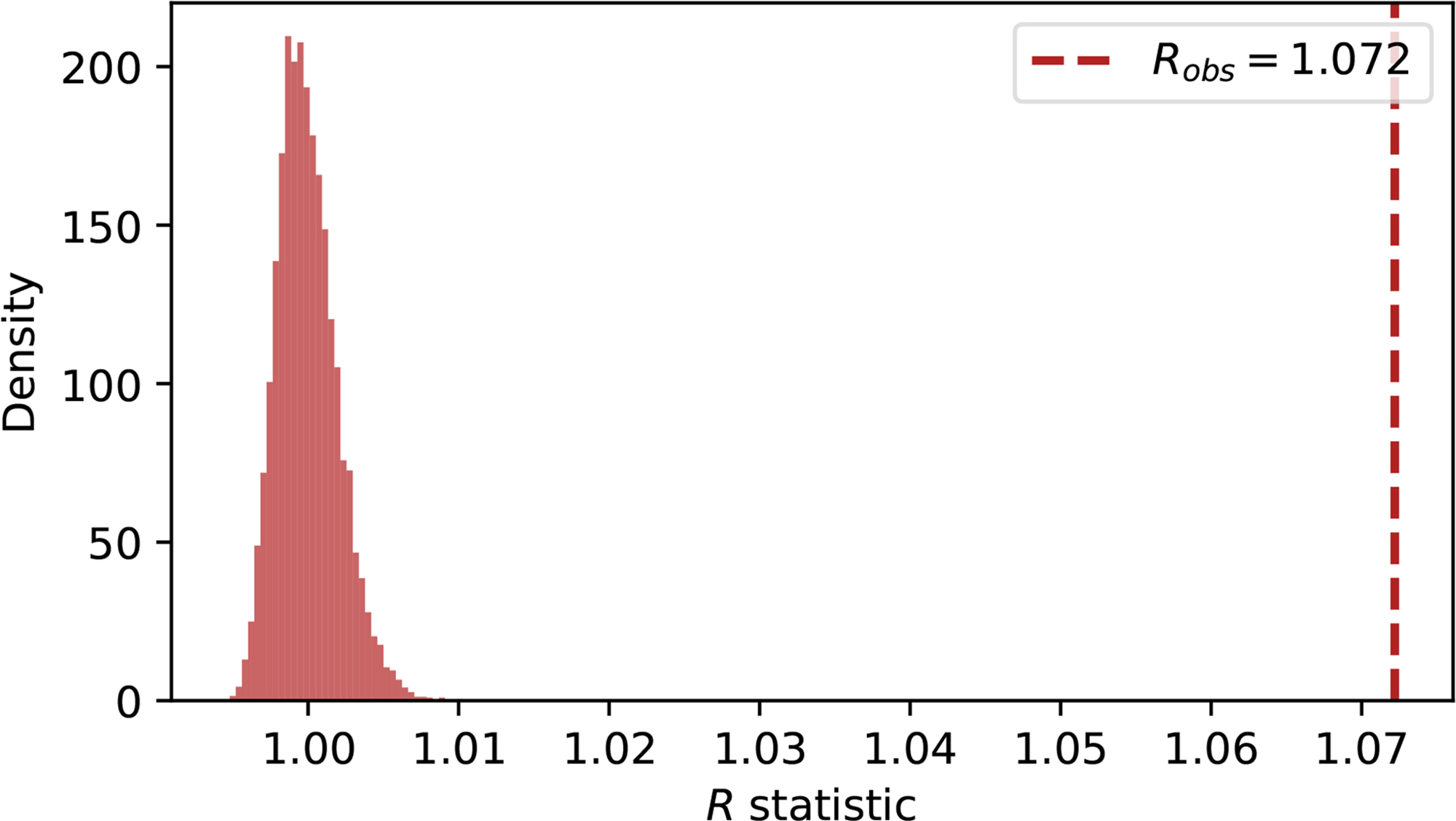
Figure 13
Empirical null distribution of the statistic obtained from permutation samples, shown as a histogram. The red vertical line indicates the observed value .