
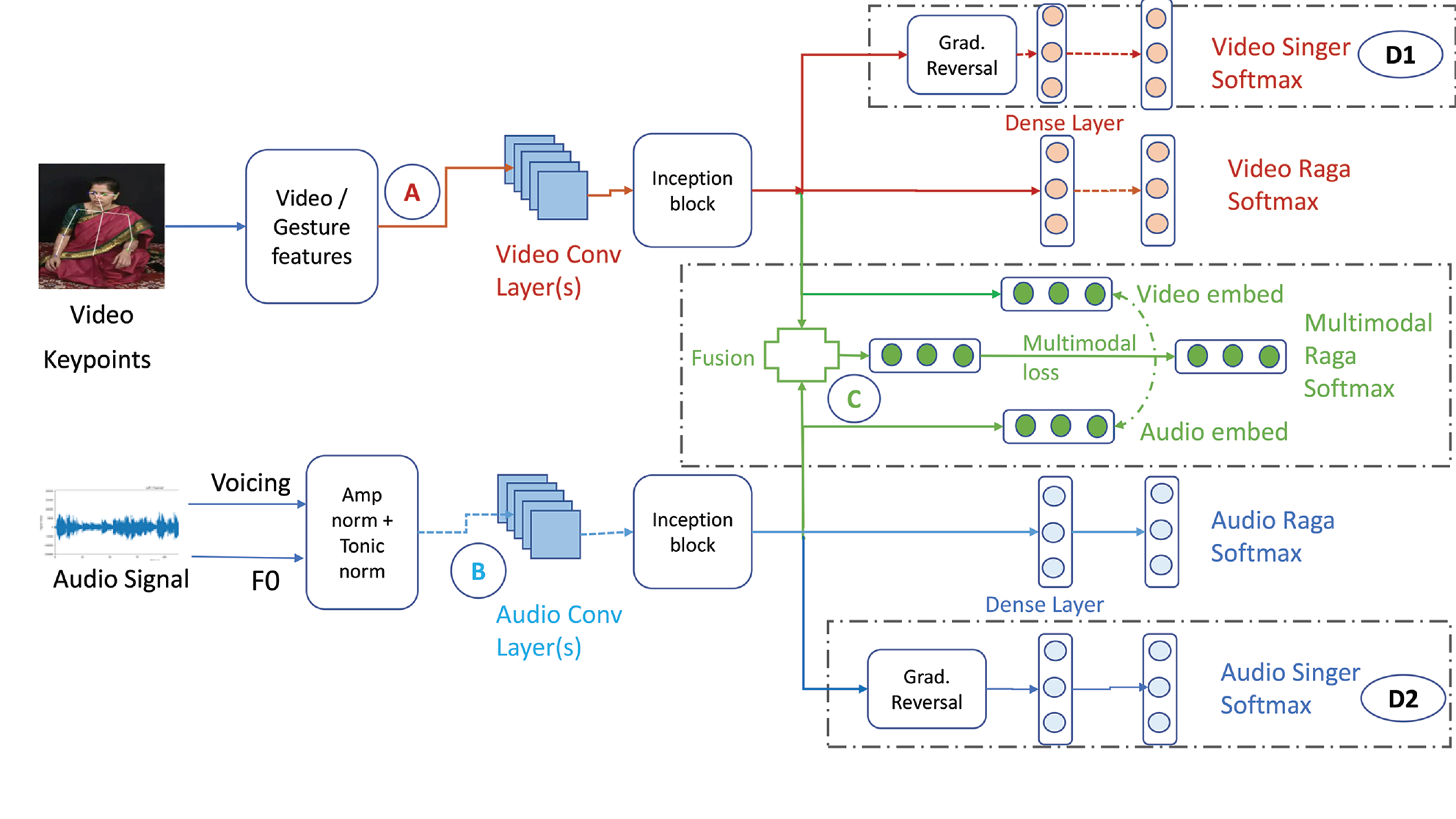
Figure 1
Proposed system for multimodal classification from pose and audio time series extracted from 12‑s video examples. We show here unimodal classification from video (A) and audio (B), including gradient reversal (GR). Blocks D1 and D2 are auxiliary blocks used in GR. GR is discussed in Section 3.3.2. (C) denotes the multimodal classification experiments, which are discussed in detail in Section 3.4.
Table 1
Summary statistics for our dataset.1
| Number of singers | 11 (5M, 6F) |
| Number of ragas | 9 |
| Number of alap recordings | 199 |
| Total recording time (mins) | 609 |
| Average time per alap (mins) | 03:18 |
Table 2
The pitch sets employed by the nine ragas.
| Raga | Scale |
|---|---|
| Bageshree (Bag) | S R g m P D n |
| Bahar | S R g m P D n N |
| Bilaskhani Todi (Bilas) | S r g m P d n |
| Jaunpuri (Jaun) | S R g m P d n |
| Kedar | S R G m M P D N |
| Marwa | S r G M D N |
| Miyan ki Malhar (MM) | S R g m P D n N |
| Nand | S R G m M P D N |
| Shree | S r G M P d N |
[i] Lower‑case letters refer to the lower (flatter) alternative; upper‑case letters refer to the higher (sharper) pitch in each case (Clayton et al., 2022).
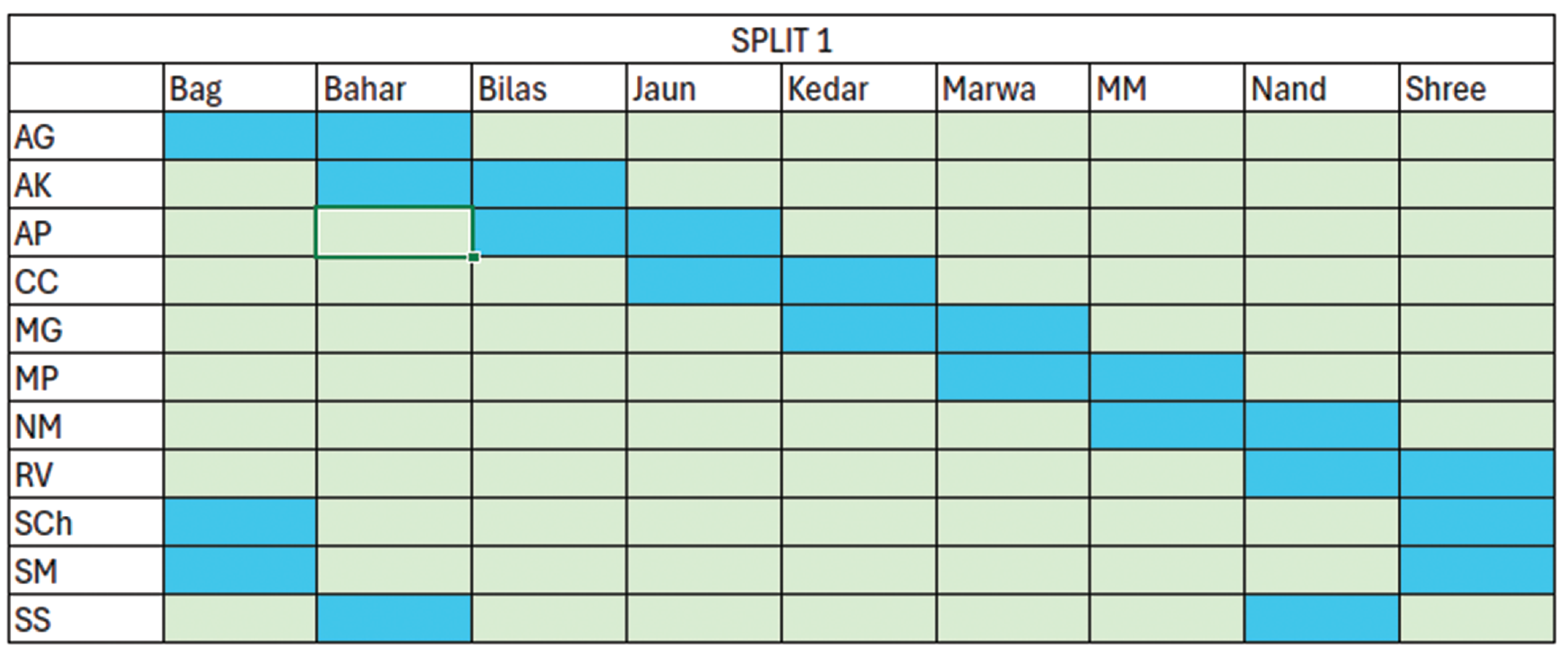
Figure 2
Schematic representation of unseen singer–raga Split 1. All 12‑s snips belonging to the green singer–raga combinations are in train and those in blue are in validation.
Table 3
Count of 12‑s segments for train and validation for the three splits.
| Total | Train | Val | Train % | Val % | |
|---|---|---|---|---|---|
| Split 1 | 18273 | 14170 | 4103 | 77.5 | 22.4 |
| Split 2 | 18273 | 14179 | 4094 | 77.5 | 22.4 |
| Split 3 | 18253 | 14269 | 4004 | 78.1 | 21.9 |
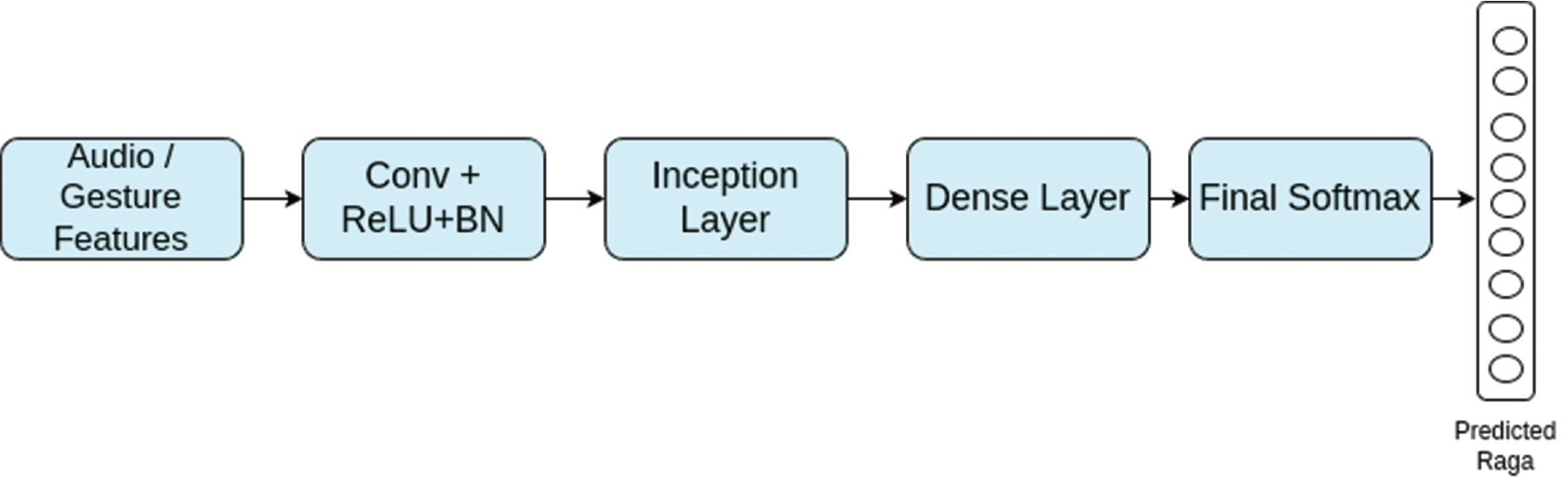
Figure 3
Architecture for unimodal classification (without gradient reversal (GR)).
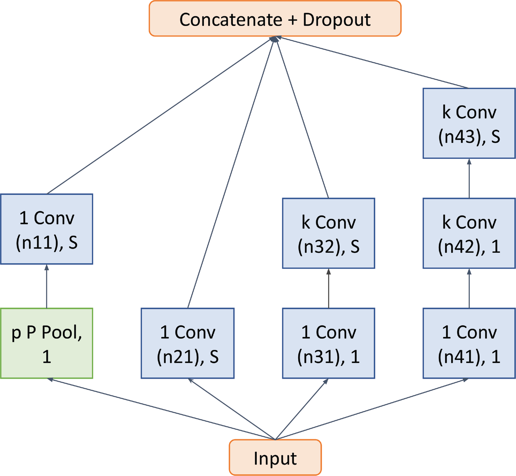
Figure 4
Detailed structure of the inception block of Figure 3. ‘k Conv (n), S’ indicates a convolution layer with n k‑sized kernels and a stride S. ‘p’ indicates the pooling size of the pool layer and ‘P’ indicates the type of pooling. k, p, P, and the number of filters were determined by hyperparameter tuning. S = 1 for the video and S = 2 for the audio model. The inception block is similar to that used in the work of Clayton et al. (2022).
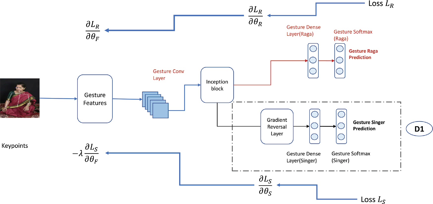
Figure 5
Gradient reversal (GR) schematic diagram—we show this with respect to gesture features. However, GR can be used even for audio features. The D1 block here corresponds to the D1 block in Figure 1. All layers are trainable.
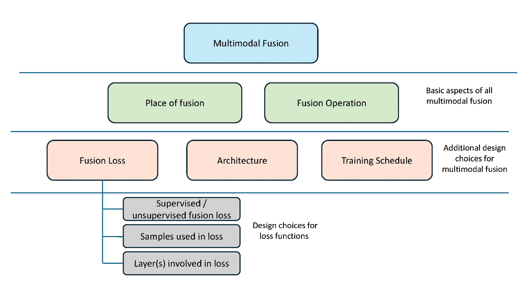
Figure 6
Proposed framework to understand the different options available in multimodal fusion.
Table 4
A framework to study the body of existing multimodal fusion techniques.
| Parameter | Options | Comments | Used in |
|---|---|---|---|
| Place of fusion | Source fusion | Fuse input features | Chen et al. (2014); Clayton et al. (2022); Gavahi et al. (2023) |
| Latent fusion | Fuse hidden layers of network | (Tang et al. 2022); Clayton et al. (2022); Jin et al. (2020) | |
| Decision fusion | Combine predictions of model | Clayton et al. (2022); Nemati et al. (2019) | |
| Operation of fusion | Concatenation | Need to have compatible dimensions | Rajinikanth et al. (2020) |
| Element‑wise addition | Raza et al. (2020) | ||
| Depthwise stacking | Chu (2024) | ||
| Include multimodal loss | No | Do not include multimodal loss | Zhou et al. (2020) |
| Yes | Choices for multimodal loss discussed later | ||
| Architecture of fusion layer | CNN‑based | CNN | Rajinikanth et al. (2020) |
| Attention‑based | Attention across fused layers | Praveen et al. (2022) | |
| Transformer‑based | Transformer‑based models | Gong et al. (2022) | |
| Training schedule | Frozen unimodal layers | Gammulle et al. (2021) | |
| Trainable unimodal layers | Li et al. (2023a) | ||
| Parts of a network | Loss is used to update weights of network parts | Yang et al. (2022) | |
| Alternate training epochs | Different epochs update different network parts | Gong et al. (2022) | |
| Multimodal loss options | Type of loss | Unsupervised—multimodal loss does not use label information | Yang et al. (2022) |
| Supervised | Franceschini et al. (2022) | ||
| Samples used in loss | Matched positive examples | Yang et al. (2022) | |
| All samples in batch | Franceschini et al. (2022); Li et al. (2023a) | ||
| Additional negative samples | Oramas et al. (2018); Puttagunta et al. (2023) | ||
| Layers used in loss | Fusion layer | Franceschini et al. (2022); Mai et al. (2022) | |
| Layer prior to fusion layer | Yang et al. (2021) | ||
| Unimodal output softmax layer | Yang et al. (2022) | ||
| Multiple layers of network | Fan et al. (2016); Wang et al. (2023) |
[i] CNN: Convolutional Neural Network
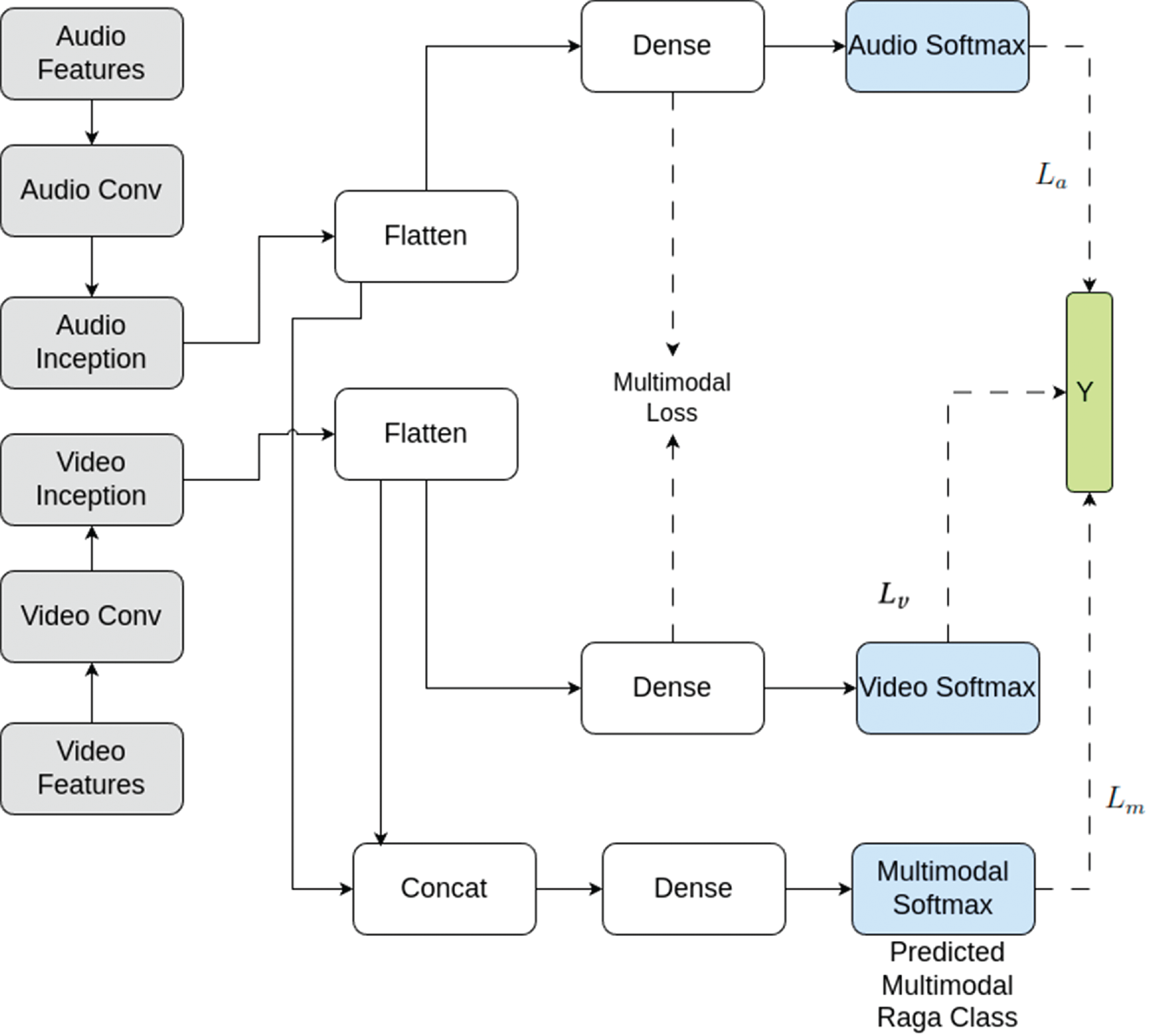
Figure 7
General structure of multimodal loss–based fusion. The blocks in grey are from the best models of the individual modalities. The grey blocks are kept frozen or trainable in various experiments. If trainable, then they are initiated from the weights of the best unimodal models. The blue boxes reflect the layers with which we compute the crossentropy losses with respect to the ground truth (shown in green). The final predicted output with respect to which we report accuracies corresponds to the multimodal softmax block. Other hidden layers part of the architecture are shown in white.
Table 5
Hyperparameter configurations for different models.
| Used in Model | Parameter | Values |
|---|---|---|
| Audio and video unimodal. source fusion, latent fusion | Temporal resolution | 10, 20 ms |
| No. of conv Layers | 1, 2 | |
| No. of conv filters | 4, 8, 16, 32, 64, 128 | |
| Kernel size | 3, 5, 7 | |
| Num inception blocks | 1 | |
| Inception_filters | 4, 8, 16, 32, 64, 128 | |
| Regularization (L2) weight | 0–1e‑4 | |
| Dropout rate | 0–0.5 | |
| Learning rate | 0.01, 0.001, 1e‑4 | |
| *Multimodal decision fusion | Support vector machine—regularizer weight | 0.01, 0.1, 1, 10, 100 |
| Support vector machine—kernel | RBF | |
| Models with multimodal loss | Common embed dimension | 2–128 |
| Temperature (only for BPCL) | 0–1 | |
| Regularization (L2) weight | 0–1e‑4 | |
| Dropout rate | 0–0.5 | |
| Learning rate | 0.01, 0.001, 1e‑4 |
[i] BPCL: Batch Pairwise Contrastive Loss
Table 6
Unimodal singer classification accuracy (%) for validation data using various features.
| Modality | Feature | Split 1 | Split 2 | Split 3 | Mean |
|---|---|---|---|---|---|
| Audio | F0+VM | 48.1 | 45.9 | 52.3 | 48.8 |
| Video | VA‑W | 88.6 | 89.6 | 89.2 | 89.1 |
| VA‑WE | 91.8 | 92.7 | 93.2 | 92.5 | |
| PVA‑W | 95.9 | 96.0 | 96.1 | 96.0 | |
| PVA‑WE | 97.8 | 97.3 | 97.4 | 97.5 |
[i] VM: Voicing Mask, P: Position, V: Velocity, A: Acceleration, W: Wrist, E: Elbow
Table 7
Unimodal accuracies (%) on validation data with and without gradient reversal (GR) for different feature combinations.
| Modality | Feature | Split1 | Split2 | Split3 | Mean | ||||
|---|---|---|---|---|---|---|---|---|---|
| Raga | Singer | Raga | Singer | Raga | Singer | Raga | Singer | ||
| Audio | F0 (RF) | 57.2 | ‑ | 56.7 | ‑ | 58.5 | ‑ | 57.4 | ‑ |
| F0 | 63.0 | ‑ | 65.8 | ‑ | 60.9 | ‑ | 63.2 | ‑ | |
| F0 + VM | 83.0 | ‑ | 84.9 | ‑ | 81.3 | ‑ | 83.1 | ‑ | |
| F0 + VM + GR | 86.1* | 13.2 | 84.3 | 11.1 | 82.7 | 11.5 | 84.3 | 11.9 | |
| Video | PVA‑WE (RF) | 10.7 | ‑ | 11.9 | ‑ | 11.0 | ‑ | 11.2 | ‑ |
| VA W | 13.8 | ‑ | 15.3 | ‑ | 14.6 | ‑ | 14.5 | ‑ | |
| VA‑W + GR | 17.8* | 11.8 | 18.0* | 12.1 | 17.0* | 14.2 | 17.6* | 12.7 | |
| VA‑WE | 14.2 | ‑ | 14.6 | ‑ | 13.4 | ‑ | 14.1 | ‑ | |
| VA‑WE + GR | 16.1* | 13.5 | 16.5* | 12.9 | 15.8 | 12.6 | 16.1* | 13.0 | |
| PVA‑W | 11.1 | ‑ | 13.7 | ‑ | 13.5 | ‑ | 12.7 | ‑ | |
| PVA‑W + GR | 17.8* | 14.2 | 17.9* | 13.8 | 17.1* | 13.5 | 17.6* | 13.8 | |
| PVA‑WE | 10.7 | ‑ | 11.5 | ‑ | 11.0 | ‑ | 11.1 | ‑ | |
| PVA‑WE + GR | 18.4* | 12.4 | 19.8* | 10.1 | 18.3* | 12.8 | 18.8* | 12.1 | |
[i] The first row in each modality results corresponds to a random forest model on the stated feature (F0 for audio, PVA‑WE for video). Singer scores are accuracies on the auxiliary singer classification arm for GR models and hence not relevant for models without GR. Bold numbers indicate the best val. accuracy for each split in each modality. Bold feature indicates the best feature in each modality by mean across splits—these models are used in multimodal experiments reported in Table 8. (*) indicates where the model with GR is statistically better () than the model without it.
[ii] GR: Gradient Reversal, VM: Voicing Mask, P: Position, V: Velocity, A: Acceleration, W: Wrist, E: Elbow
Table 8
Different multimodal fusion approaches and their split‑wise validation accuracies.
| Model | Place of fusion | Training Schedule | Multimodal Loss | Accuracies(%) | |||||
|---|---|---|---|---|---|---|---|---|---|
| Unimodal weights | Layers updated by multimodal loss | Type of loss | Samples used in loss | Split 1 | Split 2 | Split 3 | Mean | ||
| SF | Raw features | Trainable | NA | 60.2 | 61.5 | 56.4 | 59.4 | ||
| DF | Unimodal softmax | Frozen | 83.7 | 86.1* | 83.2 | 84.3 | |||
| LF | Conv. O/P | Frozen conv. | 76.1 | 73.6 | 73.0 | 74.2 | |||
| MCL | Inception O/P | Trainable conv. + inception | Both modalities | Unsup. | Paired | 78.9 | 79.1 | 80.1 | 79.4 |
| Video | Unsup. | Paired | 79.1 | 79.3 | 80.5 | 79.6 | |||
| Frozen conv. + inception | Both Modalities | Unsup. | Paired | 87.6* | 86.4 | 83.1 | 85.7* | ||
| Video | Unsup. | Paired | 87.8* | 86.5* | 83.5 | 86.0* | |||
| MCL + NS | Inception O/P | Frozen conv. + inception | Video | Unsup. | Paired + random Vec. | 80.4 | 79.5 | 79.9 | 79.9 |
| Sup. | Paired + neg. | 86.9* | 84.9 | 82.4 | 84.7 | ||||
| Sup. | Paired + hard neg. | 87.1* | 85.5 | 82.6 | 85.1 | ||||
| BPCL | Inception O/P | Frozen conv. + inception | Both modalities | Unsup. | All samples in batch | 87.9* | 86.1* | 84.7* | 86.2* |
[i] For latent fusion, operation of fusion is depthwise stacking; for all others, it is concatenation. Except for source fusion, weights of best unimodal models including gradient reversal (GR) are either frozen or trainable layers initialized with them. The best unimodal models from Table 7 are ‘F0 + VM + GR’ and ‘PVA‑WE + GR’ for audio and video, respectively. (*) indicates where the multimodal model results are statistically better () than the corresponding results for audio alone. Bold indicates the best‑performing model for that split.
[ii] SF: Source Fusion, LF: Latent Fusion, DF: Decision Fusion, MCL: Multimodal Contrastive Loss, MCL + NS: Multimodal Contrastive Loss with Negative Sampling, BPCL: Batch Pairwise Contrastive Loss
Table 9
Average accuracy (%) across 30 splits. (*) indicates statistically significant with respect to audio ().
| Split Type | Audio (%) | Video (%) | MM (%) |
|---|---|---|---|
| Addl‑Splits | 78.7 | 19.8 | 80.4* |
| Test‑Splits | 76.0 | 12.9 | 77.1* |
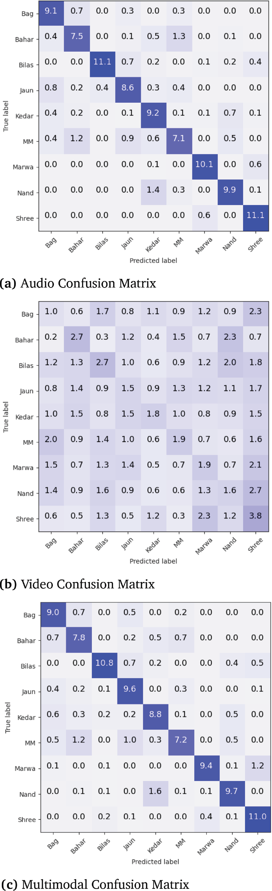
Figure 8
Normalized confusion matrices on validation data across three splits. Numbers represent percentage of the total validation data. The models are the best unimodal and multimodal models viz. F0 + VM + GR for audio, PVA‑WE + GR for video, and BPCL for multimodal.
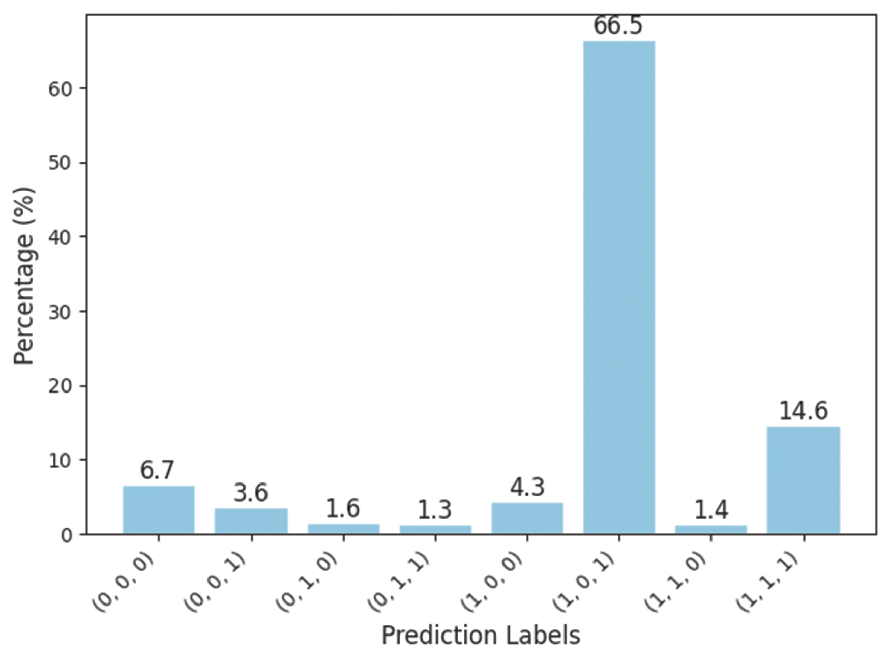
Figure 9
Histogram indicating percentage of the validation data predicted correctly (1) or incorrectly (0) by audio, video, and multimodal models. For example, 011 indicates incorrect prediction by audio but correct predictions by video and multimodal classifiers. The models are the best unimodal and multimodal models viz. F0 + VM + GR for audio, PVA‑WE + GR for video, and BPCL for multimodal.
Table 10
Accuracy (%) for 12‑s tokens with total silence duration greater/less than 2 s across the validation data of three splits.
| Silence | % Samples | Audio | Video | MM |
|---|---|---|---|---|
| <=2s | 84.6 | 86.3 | 18.7 | 87.7* |
| >2s | 15.4 | 73.3 | 19.0 | 77.6** |
| Overall | 100.0 | 84.3 | 18.8 | 86.2* |
[i] (*) denotes multimodal accuracy is better than audio accuracy with , (**) indicates .