
Figure 1
An example of the wavetables we use (before normalisation and peak alignment), corresponding to matrix with .
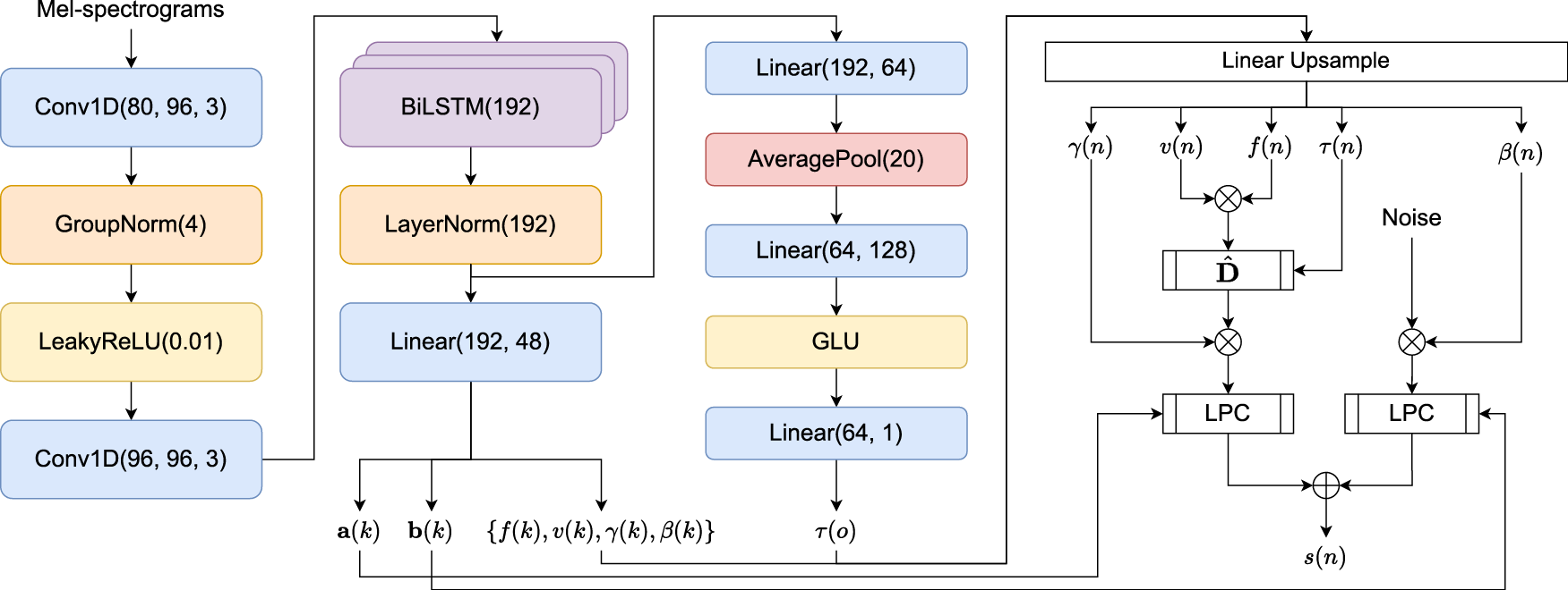
Figure 2
Overview of the GOLF synthesis process.
Table 1
Evaluation results on the test set. The lower, the better. We omit the standard deviation which is less than 0.01.
| Singers | Models | MSSTFT () | MAE‑f0 (cent, ) | FAD () |
|---|---|---|---|---|
| f1 | DDSP | 3.09 | 74.47 1.19 | 0.47 0.03 |
| SawSing | 3.12 | 78.91 1.18 | 0.32 0.01 | |
| GOLF | 3.21 | 77.06 0.88 | 0.59 0.04 | |
| PULF | 3.27 | 76.90 1.11 | 0.76 0.03 | |
| m1 | DDSP | 3.12 | 52.95 1.03 | 0.56 0.02 |
| SawSing | 3.13 | 56.46 1.04 | 0.44 0.01 | |
| GOLF | 3.26 | 54.09 0.30 | 0.74 0.02 | |
| PULF | 3.35 | 54.60 0.73 | 1.26 0.03 |
Table 2
The required number of VRAM (GB) for training with a batch size of 32, real‑time factor (RTF).
| Models | Memory () | RTF () | |
|---|---|---|---|
| GPU | CPU | ||
| DDSP | 7.3 | 0.015 | 0.237 |
| SawSing | 7.3 | 0.015 | 0.240 |
| GOLF | 2.6 | 0.009 | 0.023 |
| PULF | 7.5 | 0.015 | 0.248 |
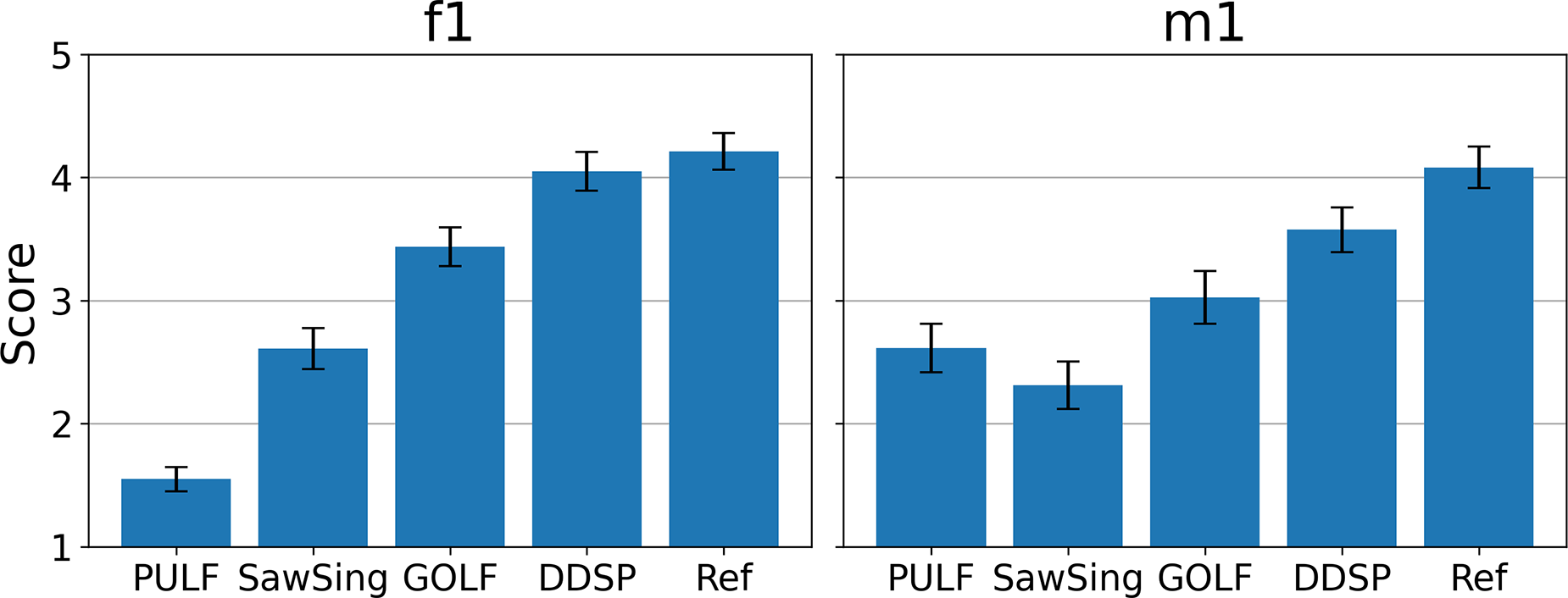
Figure 3
The MUSHRA results of the vocoders trained on different singers with 95% confidence interval.
Table 3
The L2 loss between the predicted waveforms and the ground truth.
| DDSP | SawSing | GOLF | PULF | |
|---|---|---|---|---|
| Min | 71.83 | 75.72 | 21.98 | 44.08 |
| Max | 88.77 | 93.16 | 64.82 | 70.59 |
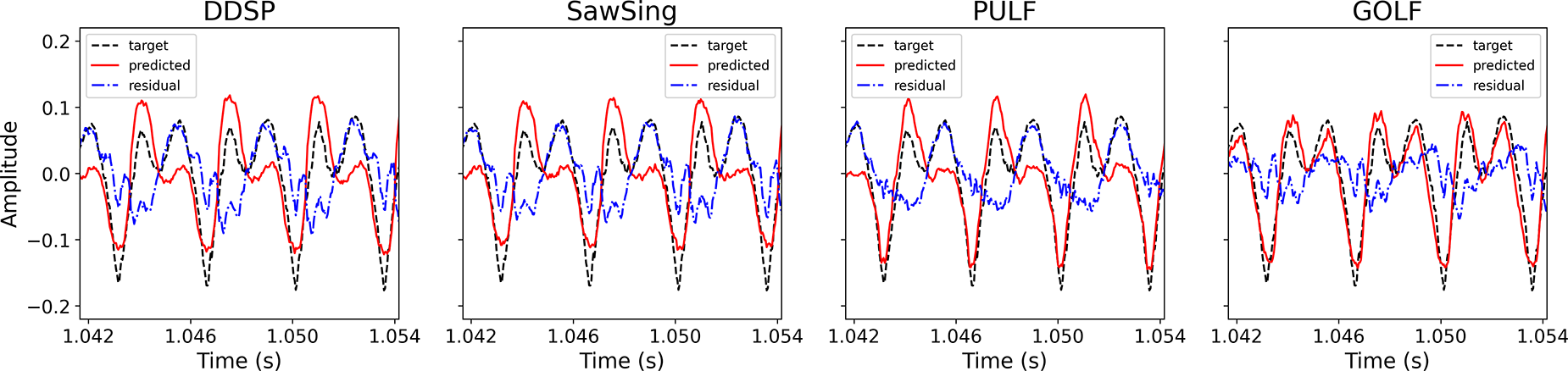
Figure 4
The predicted waveforms of a short segment from one of the m1 test samples (77 s 84 s, m1_003).
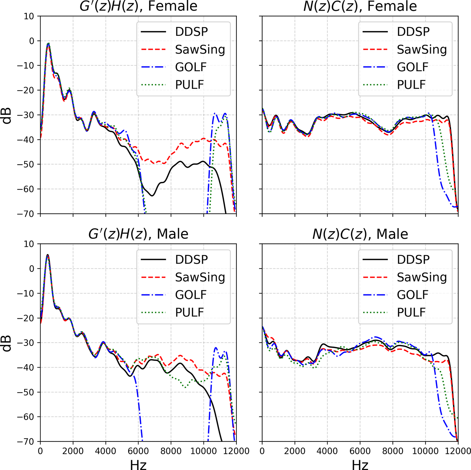
Figure 5
The average spectrums of the harmonics and noise components throughout the test set, further smoothed using cepstrum spectral analysis. The FFT size is 1024, and the hop size is 256.
Table 4
The cosine distance between harmonics and noise magnitude spectrograms of each baseline on the test data (the distance is computed only on the frequency bins below 6 kHz to avoid the frequency cut issues discussed in Section 7.2).
| DDSP | SawSing | GOLF | PULF | |
|---|---|---|---|---|
| f1 | 0.945 | 0.933 | 0.948 | 0.954 |
| m1 | 0.911 | 0.876 | 0.937 | 0.941 |
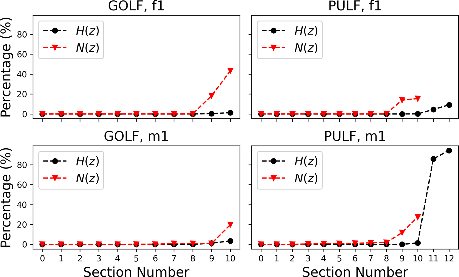
Figure 6
The portion of time occurrence of real poles of each ‑order filter in the LPC filters. For , only the frames when are considered. We sort the filters on the basis of their portion of real poles.
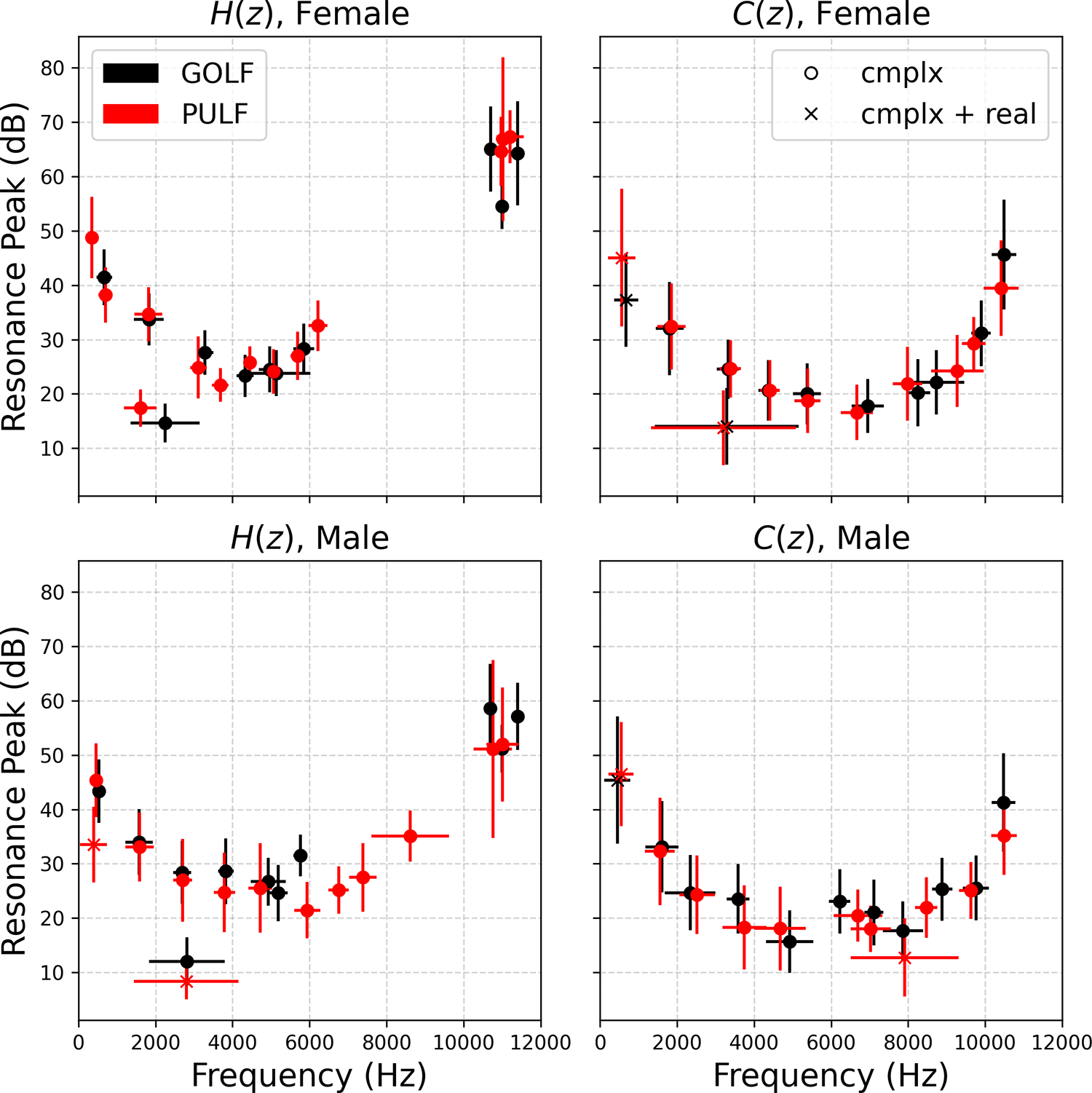
Figure 7
The mean and standard deviation of the resonant frequencies and resonant gains of each ‑order filter in the LPC filters. cmplx means filters contain real poles less than 10% of the time and cmplx + real means the opposite. The statistics are computed only on the frames when the poles are complex conjugate. For , only the frames when are considered.
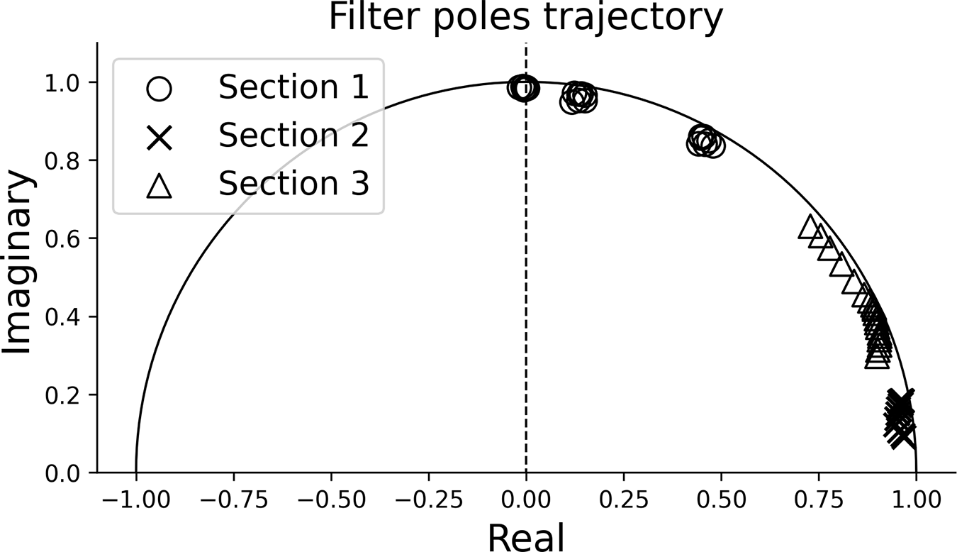
Figure 8
The trajectories of the poles of three filter sections in the LPC filters of GOLF on a slice of 0.1‑second (20 frames) test data of the f1 singer. Filter sections 2 and 3 correspond to formants and , respectively.
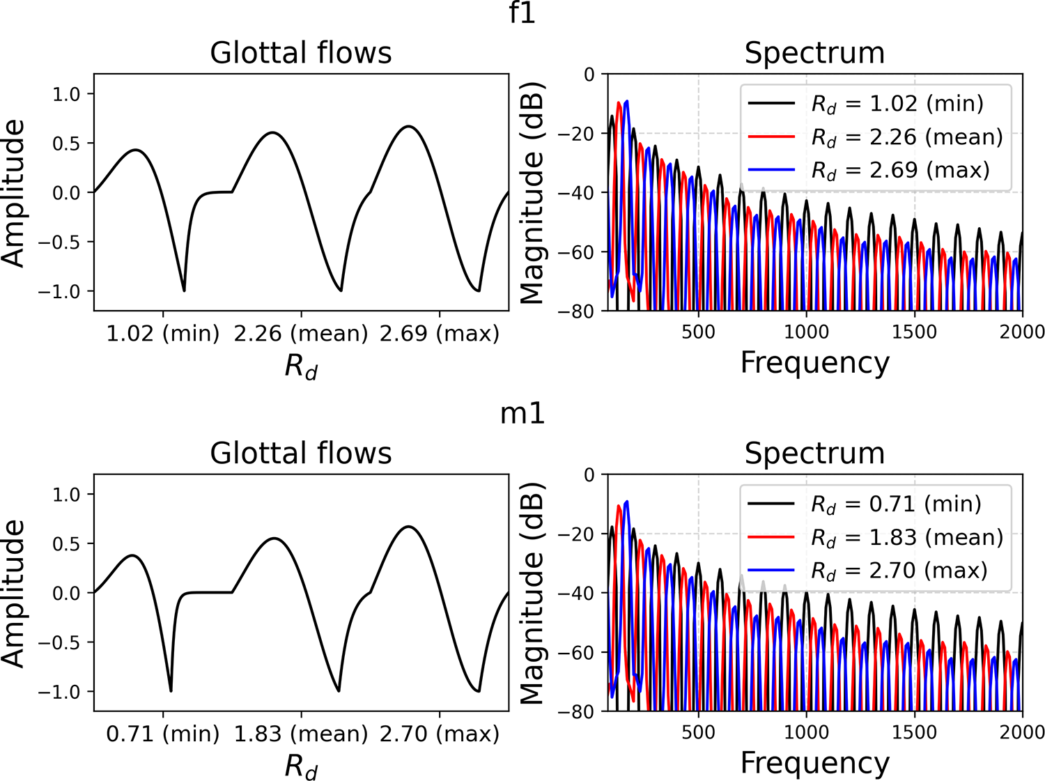
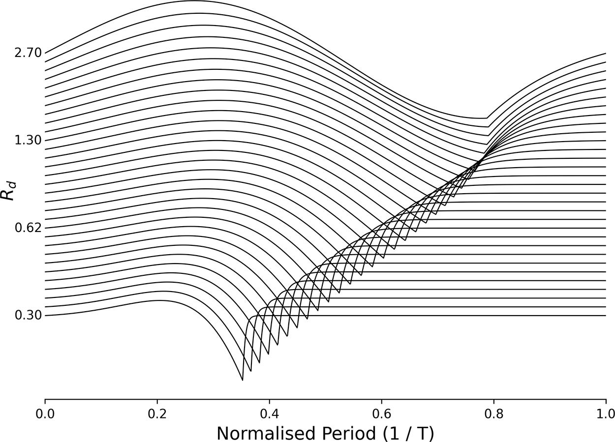
Figure 9
The glottal flows computed using the minimum, maximum and average of the values of the singers, plotted in both the time and frequency domain. The f0 for the frequency plots is set to 100 Hz, and the flows are multiplied by complex sinusoidals so the harmonic peaks are separated in the plots.