
1. Introduction
Music encoding and representation are fundamental to the design of automatic music composition systems. These choices not only affect the data structures and algorithms used for training and inference but also determine the final output format and its interaction with human users. In this paper, we propose a framework specifically designed for modeling polyphonic music originally written in Western staff notation.
1.1 Background
1.1.1 Music representation
Musical instrument digital interface (MIDI) is the most commonly used music encoding for automatic composition systems owing to its simplicity, precise timing control, and straightforward mapping to physical events. Regarding readability, for simple pieces such as a monophonic nursery rhyme, the MIDI format can be read by musicians after being rendered as the piano roll representation, or converted to modern staff notation with music engraving software quite easily. However, for complex pieces such as orchestral works, it is impossible for musicians to read piano rolls, and it is not straightforward for music engraving software to infer the modern staff notation for musicians to read. Furthermore, MIDI notation lacks musically meaningful information that can be important in music modeling and composition. For example, it does not encode pitch spellings, which are informative of the tonal context, nor does it convey metrical structures that can be reflected through note ties. Both aspects have been ignored by most existing automatic music composition systems.
Existing approaches for representing polyphonic music, primarily designed for MIDI, can be categorized as event‑based or grid‑based.
The event‑based approach (Bretan et al., 2016; Dong et al., 2023; Ens and Pasquier, 2020; Huang et al., 2019; Huang and Yang, 2020; Jaques et al., 2017; Roberts et al., 2018; Suzuki, 2022; Walder, 2016) encodes music as a sequence of note events. This encoding works straightforwardly for monophonic melodies, as note events are naturally ordered in time. However, it is not obvious when it comes to polyphonic music, where note events can occur simultaneously. One can choose to merge all events from multiple streams into a single sequence following a specific order and with additional control tokens. This is a procedure often referred to as linearization of structured data. Examples include the sequence of predefined event types as in MIDI Type 0, and similar representations as in Simon and Oore (2017) and Huang et al. (2019). The resulting sequence, however, is often very long and loses composability between parts or streams. Another way is to define a vocabulary of symbols such that polyphonic pieces can be represented as a monophonic stream. For example, one can segment the time axis at note onsets and offsets, with each segment treated as an “event” token and represented with a ‑hot vector (Walder, 2016) indicating possible active pitches. This method results in shorter sequences in general; however, it comes with a large vocabulary size that is exponential to the number of simultaneous notes, which may result in data sparsity issues. Also, as all parts are mixed together using combined tokens, certain composability and dynamics between different parts are missing.
The grid‑based approach discretizes the time dimension into a uniform grid with a unit duration, e.g., an eighth or sixteenth note duration, as the step size (Hadjeres et al., 2017; Huang et al., 2017; Jiang et al., 2020; Yan et al., 2018). This representation makes it easy to align multiple parts of polyphonic music. However, as rhythm becomes complex, the grid size needs to be very small, making the entire grid prohibitively dense and large. For example, to authentically represent (and reconstruct) Mozart’s string quartet, K.387, third movement, one would need at least 48 steps for a single quarter note, as there are sixty‑fourth notes in one voice against sixteenth triplets in another voice. As a trade‑off for fitting in a coarser and smaller grid, the music content needs to be simplified, and an authentic representation of the original content is impossible. Some extensions, such as introducing real‑valued position offsets (Gillick et al., 2021), have been proposed for specific contexts such as drum modeling but do not generalize to other scenarios.
1.1.2 Hierarchical representation of music
Music compositions can be quite long, which poses a challenge for encoding long‑term dependencies. In response to this, researchers have considered using measures as important units for sequence modeling. For example, Bretan et al. (2016) directly sequenced measures for monophonic music generation. Other works (Mittal et al., 2021; Pati et al., 2019; Roberts et al., 2018; von Rütte et al., 2023) propose grouping notes into measures on the basis of their temporal positions and modeling hierarchical structures of music accordingly.
However, these measure models do not represent the detailed hierarchical structure within a measure as defined by modern staff notation. Their motivation differs from our work in that we aim to directly model and utilize the intricate structural elements of modern staff notation, while they focus on dealing with long context.
1.2 Proposed key idea
We observe that a score in modern staff notation is represented as a grid of part‑wise measures (Figure 1), where: (1) measures provide natural synchronization points between parts, (2) measures encode the recurring accent patterns underlying the metrical structure of the music, and (3) most notational elements of modern staff notation are organized hierarchically within a part‑wise measure. These observations motivate our design of a structured measure encoder–decoder (Section 2) that directly corresponds to the object hierarchy (measure, voice, chord/note) in modern staff notation to handle its complexities. Specifically, for processing or generation, event‑based representations are used within the measure hierarchy, while across measures, the encoded representation forms a grid.
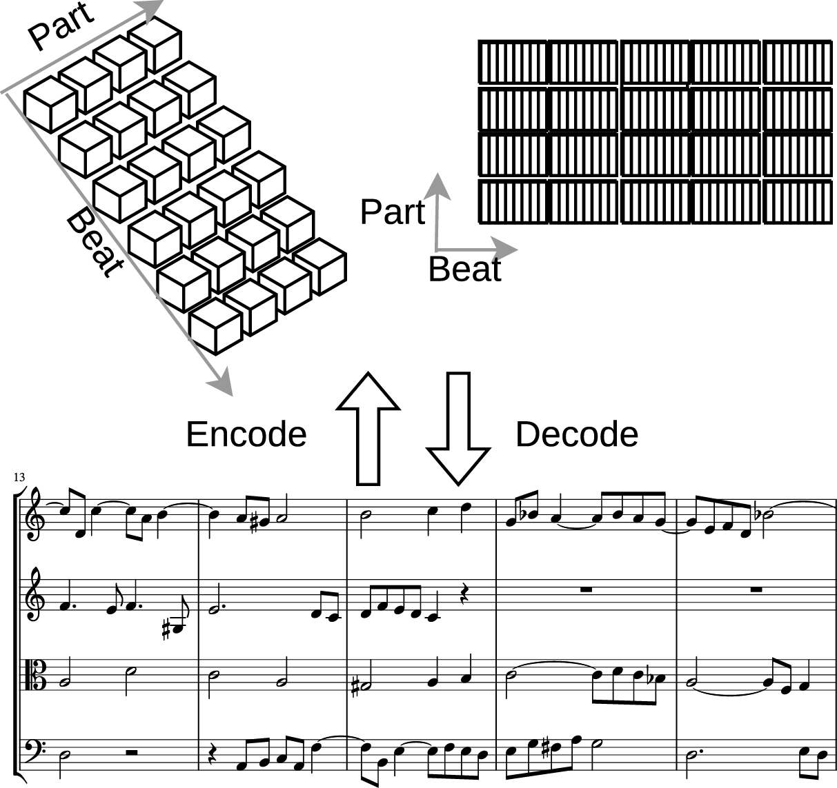
Figure 1
Overview of the proposed approach. The measure encoder encodes the entire piece into a grid, where each cell contains a vector summarizing the content of a measure within a part (left) and a matrix capturing the detailed structure of the measure (right). The example score is from J.S. Bach’s Art of Fugue.
As a proof of concept, our approach focuses on representing the core elements of staff notation necessary for forming a logical abstraction of modern staff notation. It is designed to be minimal yet extensible. Some low‑level layout details (e.g., beam slants, stem directions, and tie curvature) are left to be inferred by the engraving engine, as they can be reliably determined from those core elements using a high‑quality music engraving engine and are typically of inconsistent quality in freely available datasets.
We target modern staff notation pieces that meet two criteria: the pieces have synchronized measure lines across different staffs, excluding compositions with unaligned measures or those unsuitable for this notation (e.g., certain free improvisations and polymeter pieces); each part‑wise measure can be accurately represented using the common object hierarchy (Figure 2).
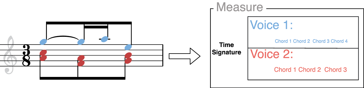
Figure 2
The common object hierarchy of a single part‑wise measure. This hierarchy specifies the compositional structure of a part‑wise measure, which includes four levels from high to low: measure, voice, chord, and note.
Encoding the score as a grid of measure representations imposes unique challenges: (1) certain alignment information between parts may get lost and (2) the decoder for each part‑wise measure must implicitly learn to perform counting, ensuring that events in each synchronous monophonic stream (voice) sum up to the same total duration.
2. Proposed Measure Model
A single part‑wise measure in modern staff notation is usually encoded to have a hierarchical structure, as shown in Figure 2, commonly utilized by music notation software (e.g., Sibelius, Finale, and Musescore) and open formats such as MusicXML. This part‑wise measure is central in forming the logical form of a music score, and is the basic unit for user interaction with notation software. From this logical form, the engraving rules (Stone, 1980) can then be implemented to determine the layout of most standardized visual elements, such as the head position, the length and direction of the stem, and the beam.
We design our measure model to reflect this hierarchy. Each part‑wise measure contains a variable number of voices. Each voice is a variable‑length sequence where each step is a chord–duration tuple. A chord is a set of notes, each of which is a pitch–tie tuple. A pitch is represented as a tuple of a diatonic step and an accidental. A tie indicates whether this note appears as a continuation of the previous note of the same pitch in the same voice. Each pitch is allowed to have its own tie status, as notationally any note of a chord can be a continuation from the previous chord. As a general treatment in this work, a chord can contain zero (rest), one (single note), or more notes. We use chord hereafter to refer to all these three circumstances. Duration is the duration of a chord as a fraction of the beat unit, which is specified by the time signature (e.g., quarter, eighth, or dotted quarter). The time signature in our model is not explicitly encoded, as it can be calculated from the beat unit and the actual number of beats within a measure. We do not directly encode the visual key signature for every measure for now, because it is not reliably encoded in the dataset.
The proposed measure model (Figure 3) is a structured encoder–decoder directly corresponding to the above hierarchy. It models four key entities: duration, chord, voice, and measure—each with a dedicated encoder–decoder pair.
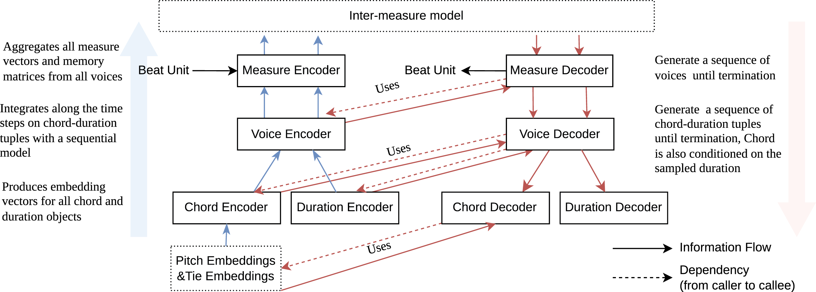
Figure 3
A high‑level illustration of the proposed measure model. The measure/voice encoder and decoder have two outputs/inputs that are vector‑valued and matrix‑valued, respectively.
All encoders aggregate information from lower‑level objects and output embedding vectors. For objects at the lowest level, i.e., pitch and tie, which have integer or boolean values, we use an embedding lookup to encode them. All decoders are autoregressive models; at each step, they invoke lower‑level objects’ decoders to generate lower‑level objects. Meanwhile, they invoke lower‑level objects’ encoders to provide vector representations of generated objects. In our experiment, we implemented autoregressive models in the measure model using gated recurrent units (GRU; Cho et al., 2014)/long short‑term memory (LSTM; Hochreiter and Schmidhuber, 1997).
Position‑Indexed Measure Memory Matrices We propose using a complementary representation in addition to the usual vector‑valued output (input) for each encoder (decoder): the voice and measure encoder (decoder) also have an additional matrix‑valued output (input) to represent position‑associated content information within the measure, taking the form of linear heteroassociative memory (Willshaw et al., 1969).
For notational convenience, throughout all levels in the hierarchy, we reuse the same symbols h and c to denote, respectively, the vector output of the encoder and the vector input to the decoder for every object’s model; we also use the same symbols M and to denote, respectively, the matrix output of the encoder and the matrix input to the decoder. The implementation details are in the supplementary material.
2.1 Preprocessing
In a diverse music corpus such as the dataset we use, there exists a large variety of time signatures, including some less common ones, such as , , and . In addition, there are often incomplete measures. These make beat counting challenging in note (chord) event generation, leading to incorrect measure lengths and desynchronization between parts. To facilitate beat counting for the measure model, we propose the following preprocessing techniques, which help generate notes with correct measure lengths, synchronize events across parts, and share patterns among sequences with different time signatures.
Padding Incomplete Measures To handle incomplete measures (e.g., pickup measures, incomplete ending measures, and incomplete measures from notating repeats), we create a padding pitch symbol, in addition to regular pitches, to complete the measure.
Duration Normalization For a given time signature, we define the beat duration as the duration of a primary division within the measure and normalize all durations accordingly. For example, in time, the beat unit is a dotted quarter note, and the measure duration is normalized to two beats. After normalization, all measures in our dataset have a length of 2 (duple), 3 (triple), or 4 (quadruple) beats. At inference time, the time signature and note durations are scaled back after generating the music content.
Cross‑Beat Note Splitting In modern staff notation (Stone, 1980), notes crossing primary divisions of a measure are conventionally split into multiple tied notes (Figure 4) to facilitate beat counting and synchronization between parts. Inspired by this practice, we split every note crossing integer beat positions into multiple tied notes. This helps the measure model count beats and synchronize between parts, and reduces the number of note durations seen by the model; for example, rare durations such as () × beatUnit are reduced to common durations, including 1 × beatUnit and × beatUnit. For reconstructing the score for rendering, these tied notes can be processed according to the desired engraving style.
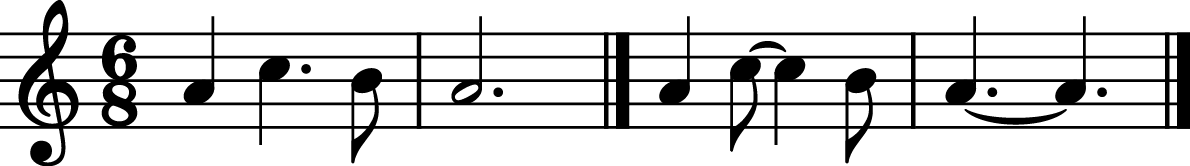
Figure 4
Example of cross‑beat note splitting, from the left two measures to the right two measures: the note C crossing the (3 + 3)/8 division is split into an eighth note and a quarter note; similarly, the dotted half note is split into two dotted quarter notes.
2.2 Chord encoder–decoder
A chord is a set of notes, each represented as a pitch–tie tuple. We encode a note as noteEmbed using element‑wise multiplication of learnable pitch and tie embeddings:
where pitchEmbed is a learnable vector for each (diatonic step, accidental) tuple, with accidental ranging from double flats to double sharps, and tieEmbed is a learnable vector for .
Chord Encoder The chord encoder computes the chord embedding by summing all note embeddings in a chord and applying a linear projection to map the sum to a desired dimension
The summation ensures that is invariant to note permutations. For an empty chord (rest), we define it as a chord containing a single (pitch = terminate, tie = false) tuple, where terminate is a special pitch symbol.
Chord Decoder The chord decoder autoregressively decodes notes (pitch–tie tuples) in an arbitrary order
where is the chord embedding, denotes note indices, and is the total number of notes. Here, the last element, pitchK, is the above‑mentioned terminate symbol.
As for decoding pitch–tie tuples, we factor the pitch–tie probability as
During training, we shuffle the order of notes in a chord.
2.3 Duration encoder–decoder
Duration Encoder In corpora with diverse note durations, less common values (e.g., double‑dotted eighth notes) create another challenge. We observe that valid durations are integer fractions (e.g., 1/2, 1/3, 3/4, and 3/2) of the beat unit. These fractions can be factorized into multiplications of small prime number exponents
where are exponents of the first several primes, and they can be positive, negative, or zero integers. We represent a duration as a ‑dimensional vector .
To cover all duration values in our dataset, we use 2, 3, 5, 7, and 11 as the prime base and as the exponent range. For example, assuming a quarter note beat unit, a dotted eighth note is of the beat unit, represented as .
The duration encoder calculates the duration embedding by concatenating digit embeddings at these exponent positions and applying a linear projection
where is a linear projection, [] is the concatenation operator, and is the shared embedding lookup function for all exponent digits .
Duration Decoder For the duration decoder, we consider the dependency between these exponents, that is, an autoregressive model of the form
2.4 Voice encoder–decoder
A part‑wise measure includes one or more voices, and each voice is a sequence of chord–duration tuples, , where denotes the index within the sequence.
Within‑Beat Position Signal as Extra Input We propose using a sinusoidal within‑beat position signal as an extra input to both the encoder and decoder at each step to facilitate beat counting:
where is the normalized onset position within a measure for step . This signal is chosen to be periodic with a period of 1 beat to avoid encoding the absolute position within a measure.
Voice Encoder To encode a single voice in a measure, we concatenate embedding vectors of chord, duration, and within‑beat position signal for each chord–duration tuple () and feed them to a bidirectional LSTM to obtain a sequence of contextual embeddings . The voice embedding vector is the mean of the contextual embeddings followed by a linear projection.
Measure Memory Matrices We run another bidirectional LSTM only with the concatenation of duration embeddings and the within‑beat position signal to obtain another sequence of contextual embeddings purely from the perspective of rhythm and position. We create a fixed‑size position‑indexed memory matrix for each voice using
where and map inputs to vectors of size memKeySize and memValSize, respectively. The resulting measure memory matrix has dimensions memKeySize memValSize.
We design several candidates for , such as:
where is a linear projection and is any activation function (e.g, identity, softmax, or sigmoid). We also consider a parametric form that directly distributes these vectors into the positions of matrices that are proportional to the beat position:
which has the shape of a skewed Gaussian distribution (skewgauss). is the position vector for every entry in the matrix, which is an equal‑distance segmentation of the measure. is the beat position for the ‑th step (a chord–duration tuple), normalized between 0 and 1 within a measure. is the sigmoid function, and , i.e., calculated from using a feedforward neural network (FNN). For val(), we use:
where is a learnable parameter. The choices of are then evaluated in Section 5.3.
This position‑indexed memory matrix can be viewed as rendering a variable‑sized feature map to a fixed‑size grid. It allows one to look back into the measure despite besides using only the summary vector . It also has the expressivity of making the alignment between voices easier: objects in different voices with a similar rhythmic context will be placed into similar columns in the matrix.
This design helps inter‑voice aggregation; column‑wise aggregation of memory matrices across voices maintains content positions and alignments.
Voice Decoder The voice decoder autoregressively generates chord–duration tuples within a voice, taking a vector and a matrix as input. It uses a separate termination predictor at each step.
At step , it first samples a duration and then conditions on the recently sampled :
Reading from the Measure Matrices At each step during decoding, the voice decoder uses a position‑dependent attention mechanism to read from the matrix‑valued input :
where , and are learnable parameters. We also consider a position‑dependent‑only variant
Certain design choices will be evaluated in Section 5.3.
2.5 Measure encoder–decoder
The measure encoder–decoder is the highest level in the measure object hierarchy. This module models a single part‑wise measure and directly interacts with the model built at the inter‑measure level.
Measure Encoder The measure encoder aggregates information from the embedding vectors and matrices of all voices in a part‑wise measure and integrates beat unit information:
where are instances of learnable embedding vectors assigned to the corresponding beat unit of the measure.
Measure Decoder The measure decoder decodes the input vector and the matrix into a beat unit and a list of arbitrary number of voices. It first generates the beat unit given c. Then, each voice is generated one by one using a GRU autoregressive model to produce the input for the voice decoder. After generating a voice, the measure decoder invokes the voice encoder to provide feedback for generating the next voice or the termination token.
3. Applications
The measure model described in Section 2 encodes and decodes a score to and from a uniform grid, serving as a versatile building block for processing music pieces written in staff notation.
3.1 Measure‑based autoregressive models
An autoregressive model factorizes the joint distribution of a sequence as
To model polyphonic music with simultaneous parts (staffs), an order should be defined to linearize the part‑wise measure sequences into a single sequence to obtain this factorization.
Linearization We linearize the grid in a column‑first manner as shown in Figure 5. To enable arbitrary ordering of parts/instruments, we shuffle part‑wise measures in each column, as demonstrated in the example.
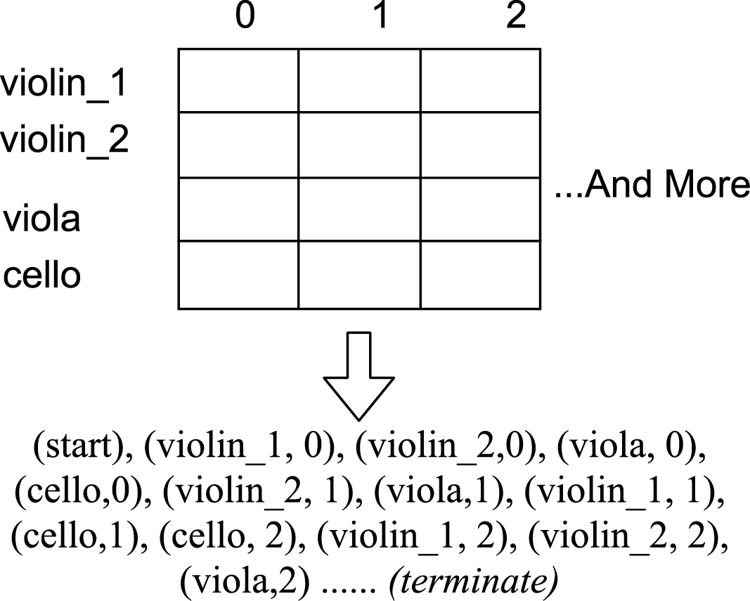
Figure 5
Linearization of the measure grid for autoregressive modeling using the measure model.
Loss Function The maximum likelihood estimation (MLE) loss function is defined as
where is the empirical data distribution; the expectation is estimated from the minibatch.
Inter‑measure Model The inter‑measure model prepares the input for the measure decoder to produce the next part‑wise measure, using the previous history of generated measures. The Measure Encoder encodes all measures in the context, and then instrument embeddings and sinusoidal position embeddings (for measure positions within a part) are added. It first uses a context model to summarize the context () as in Equation 17. This context model uses relative self‑attention layers similar to Shaw et al. (2018) and Huang et al. (2019). The attention score computation incorporates the regular inner product, relative distances of measure indices (all parts together) and relative distances of vertical (single‑part) measure positions, and an indicator term for whether measures are in the same part (staff). For conditioning the next part‑wise measure generation on a specific part, the instrument token and position embedding of the next part‑wise measure are fed to another set of relative attention blocks with cross‑attention to the context vectors. The output vector serves as an input for the measure decoder to generate the next part‑wise measure.
Measure Memory Aggregation Additionally, a matrix produced by aggregating measure matrices at the same vertical position is fed to the measure decoder as a local reference
where is the corresponding vertical position index of part‑wise measure . Further details are provided in the supplementary material.
3.2 Measure‑based conditionally specified distributions (CSD)
Another paradigm models joint distributions of multiple variables (in this work, measures on the grid) as a set of conditional distributions, where the consistency/compatibility between these conditional distributions is not required.1 Such models are called conditionally specified distributions (CSD; Arnold et al., 2001; Van Buuren et al., 2006) or dependency networks (Heckerman et al., 2000). Order‑agnostic models (Germain et al., 2015; Uria et al., 2014; 2016) seek to learn a set of weight‑shared autoregressive models under an arbitrary generation order, which can be viewed as a special case of conditionally specified distributions.
Inference/sampling from conditionally specified distributions is performed by sampling from different conditionals, either iteratively (e.g., pseudo‑Gibbs sampling, starting from some initialization of all positions) or non‑iteratively (e.g., order‑agnostic autoregressive models, filling all positions in one pass with some ordering). In this case, the actual distribution from which the model samples is implicitly specified by both these conditional distributions and sampling procedure. This paradigm has been used for data imputation (Van Buuren et al., 2006), language models (Devlin et al., 2019), and music generation (Hadjeres et al., 2017; Huang et al., 2017; Yan et al., 2018), etc.
Advantages of CSD include the following: (1) It allows more flexible conditioning by treating any given variables as conditions. (2) It improves generalization, as it forms an implicit ensemble (see Uria et al. (2016), and also note its similarity to the token drop mechanism [Kågebäck and Salomonsson, 2016; Sennrich et al., 2016; Zhang et al., 2020] from the aspect of regularization). (3) It provides flexibility from specifying entire factorized joint distributions to only local conditional distributions given all other variables, as in many cases the conditional distribution is simpler and more deterministic when more observations are given as conditionals.
To apply this paradigm to automatic music composition, one needs to know the number of positions to make predictions so that generation can proceed to arbitrary positions. This creates no difficulty for models that discretize the entire score with a fixed step size (Hadjeres et al., 2017; Yan et al., 2018); however, as shown previously, the grid can be too fine for polyphonic pieces with diverse rhythmic values. For approaches using event‑based encoding, a vanilla choice is to fix the number of note events in the piece or to use a non‑trivial dedicated model dealing with variable sequence length. For both approaches based on the grid‑based and the event‑based encodings, the representations are too fine to perform sweeps of iterative sampling, as it requires more iterations, and each iteration requires invoking the entire deep neural architecture (e.g., self‑attention layers).
Applying CSD is one of the main motivations for this work. We view the measure model as a convenient way to adapt this paradigm to corpora of rhythmically complex and long musical pieces that have a variable number of parts. The measure model defines the number of positions according to the natural segmentation unit in modern staff notation (measures), providing a musically inspired basis for arbitrary‑order iterative sampling, that imitates the organization basis for human composers working with a score.
Masked Conditional Specification As illustrated in Figure 6, we specify the conditional distributions as follows:
where is a part‑wise measure that is masked and is the measure grid. We use to represent the masking operation with the binary mask Mask. The masking operation is implemented by substituting the encoding vectors of masked measures with a trainable vector and, meanwhile, zeroing out the corresponding measure memory matrices.
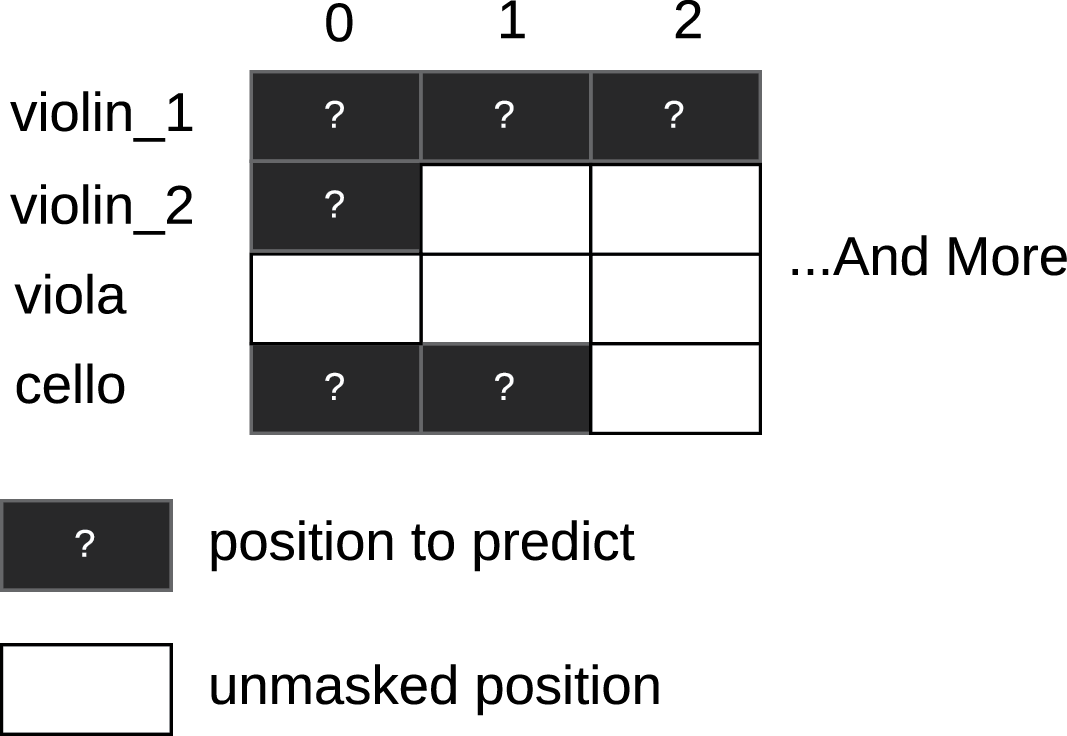
Figure 6
Masked conditional specification.
Loss Function The loss function is a weighted sum of conditional log‑likelihoods, technically called a composite log‑likelihood function. It is interesting that different weighting schemes lead to different proper scoring rules. Uria et al. (2016) apply a weight that makes the loss identical in expectation to the expected log‑likelihood of the autoregressive model over uniformly sampled orders. We rewrite this in an equivalent form adapted to our case:
where is the total number of part‑wise measures and |Mask| is the number of masked measures. Here, the number of masked measures is sampled uniformly. However, with this weighting, if the mask contains only one position to predict and the piece has several thousand part‑wise measures, this single measure receives a weight of thousands, making the gradient unbalanced. To mitigate this, we propose the following loss as an approximation to importance sampling of Equation 21:
where is the batch size and is generated by sampling the ratio of masked positions from , which can be sampled via .2 We also found adding a handy reconstruction loss of unmasked measures helpful in end‑to‑end training and regularizing the measure model when paired with corruption of unmasked measures during training (token drop, pitch distort, duration distort, etc.):
Then, the final loss is
where is a scalar. One special case is that, when the loss is identical to the denoising autoencoder.
Inter‑measure Model The inter‑measure model for masked conditionals takes as input the encoded measure grid, instrument embeddings, and position embeddings. The outputs at the corresponding positions are used as inputs to the measure decoder. In addition, we sum measure memory matrices at the same simultaneous (vertical) measure position as the matrix input to the measure decoder. We use dilated hybrid LSTM/relative self‑attention layers for the inter‑measure context model. Further details about the architecture of the inter‑measure model used in the experiment are provided in the supplementary material.
Generation Procedure This paradigm allows for flexibility in designing the inference/generation procedure, and we present one such procedure in Alg. 1. We initialize the entire score by masking the entire score and filling masked positions (measures) one by one, similar to the procedure in Huang et al. (2017).

Algorithm 1:
Sampling/Inference procedure
A refinement stage can be included after the initial pass, which iteratively masks and fills a random portion of positions to refine the already‑filled score. If the set of masked positions only contains one position in the refinement stage, it is referred to as pseudo‑Gibbs sampling. In such cases, the algorithm makes small moves in the data space, which can cause slow mixing time and make the sampling procedure get stuck at spurious stable local patterns. Masking more positions at a time can effectively create larger moves in the data space.
For conditional generation, certain measures given as conditions are kept intact during initialization and refinement.
4. Comparison with Related Works
The multitrack music transformer (MTMT; Dong et al., 2023) is a transformer‑based autoregressive (AR) model on a MIDI note event sequence. This model is similar to our AR baseline model, which will be described in the experiment section, in the sense that, in sampling each note event, it also samples which instrument a certain note belongs to; in this way, the model achieves the goal of generation of music with variable instrumentation. Different from Dong et al. (2023), our AR baseline model also considers the dependencies between different attributes (duration, pitch, and instrument [part]) of the note events. To support multipart functionality, the AR Measure model in Section 3.1 does not need to predict certain instrument (part) labels, as it autoregresses over a grid of part‑wise measures, where the instrumentation is provided as conditions.
Coconet (Huang et al., 2017), a convolutional neural‑network‑based music generation system, also falls under the CSD paradigm, more specifically, the neural autoregressive distribution estimation (NADE) approach (Uria et al., 2016). The key difference is that Coconet uses a fixed grid by discretizing score positions, while our CSD model described in Section 3.2 is based on a grid of part‑wise measures, with each cell representing a structured part‑wise measure object handled by the proposed measure model. Consistent with our notation, the training objective in Coconet is
Our Equation 21 differs from Equation 25 by a factor of , the number of grid positions, because Coconet uses a fixed grid size, while our approach handles variable‑sized grids.
5. Experiment and Evaluation
5.1 Dataset
We used MusicXML as the input score format, requiring all pieces to be well formed in the following sense: (1) all durations in a voice sum up to the same number of beats indicated by the time signature, and (2) all synchronized voices/parts contain the same number of beats. A large portion of MusicXML files available online violate these constraints due to historically buggy implementations of MusicXML exportation in almost all music notation software (e.g., Sibelius, Finale, and Musescore). Therefore, we created our own dataset to ensure the cleanness of the data. The dataset includes Mozart quartets, Beethoven quartets, Corelli trio sonatas, Bach inventions, and fugues in Bach’s Well‑Tempered Clavier. The MusicXML files were converted from scores on KernScore (http://kern.humdrum.org) and manually corrected. We corrected all wrongly tied notes (e.g., slurs mistaken as ties) and wrongly quantized notes (due to the design of humdrum) for Mozart/Beethoven quartets according to the original scores. The dataset also included Bach’s Musical Offering (BWV 1079), The Art of Fugue (BWV 1080), and some movements of the Brandenburg Concertos, and eight other Baroque instrumental pieces that we collected online. The data set also includes Bach’s 371 chorales, including the one with five parts usually omitted. In total, our dataset has 847 pieces with 46,724 measures or 202,766 part‑wise measures. To correctly handle repeat signs, we created both non‑repeat and repeat versions of the scores. For the non‑repeat versions, we only expanded the Da Capo signs and not other repeats, while for the repeat version, we expanded all repeat signs. Figure 7 shows the summary statistics of the dataset on length versus number of parts and note events.
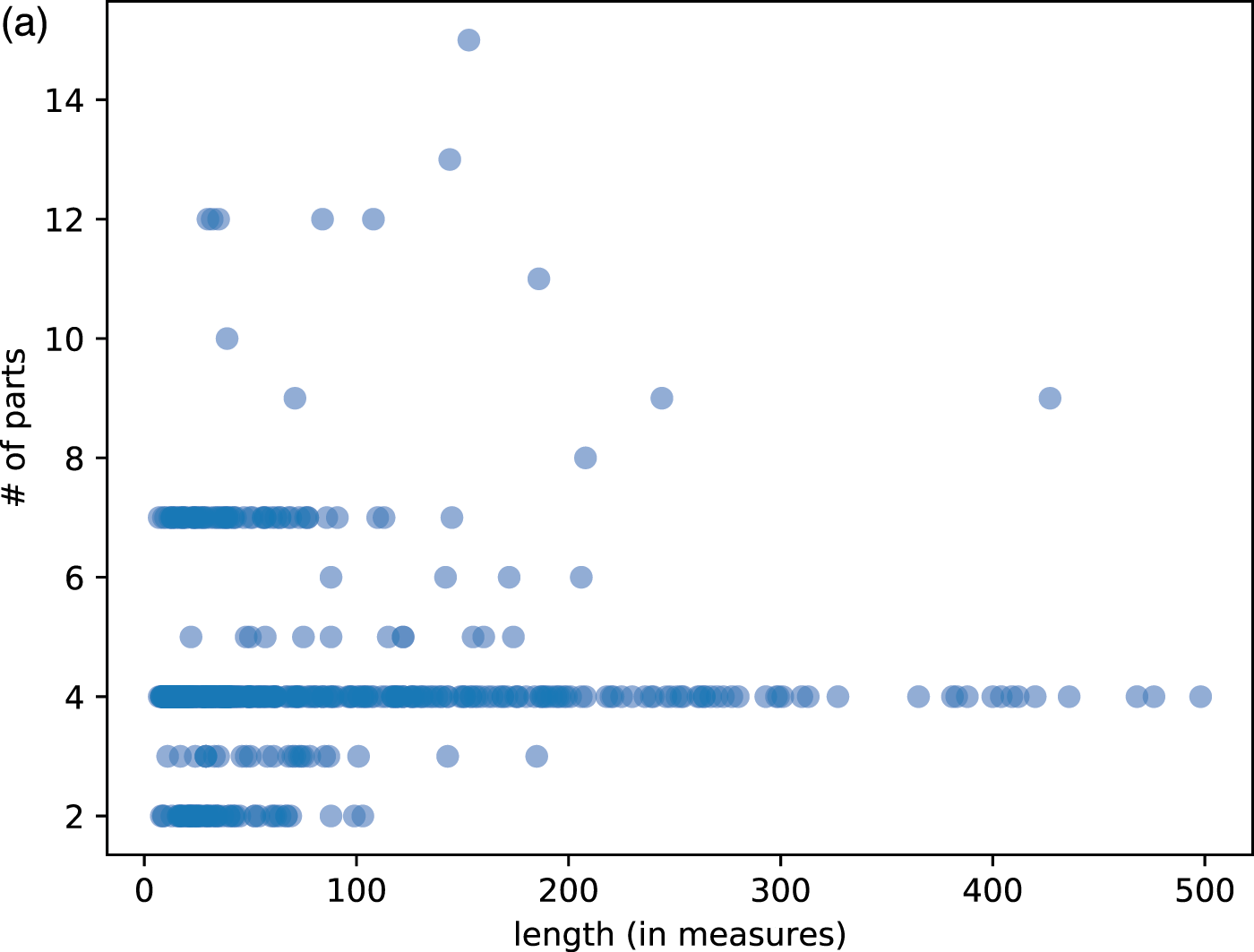
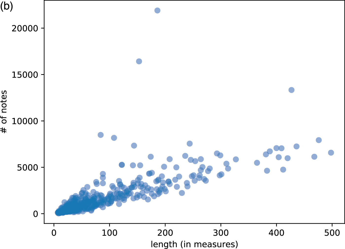
Figure 7
Some statistics of music pieces in our dataset. Each dot represents a piece. (a) Length versus number of parts (staffs). (b) Length versus number of note events.
5.2 Data augmentation
We applied key transposition to augment our dataset. However, a large shift could cause issues with some instruments’ pitch range during generation. To address this issue, we made the model aware of the transposition augmentation by renaming the instrument token of each part with a combination of the original instrument token and the amount of shift applied during transposition. For example, for a “violin” part that is shifted down by seven semitones, the new instrument token would become “violin_shifted‑7”. For transposition, note spellings were resolved to those that would create the least number of accidentals.
5.3 Ablation studies of the measure model
We evaluated some specific design choices, namely, within‑beat position signals and measure memory matrices, previously mentioned in Section 2. We expected that they could help the system better align concurrent note events from different staffs (parts) and keep the generated duration sequences summed up to the correct length. To validate this hypothesis under limited resources, we performed a simplified task that only tried to predict concurrent measures given other measures, where the sum aggregation of concurrent measures was used for both the measure vectors and the measure matrices to form the input to the measure decoder.
We first evaluated the choice of the encoding key function as used in Equation 9 (writer) and the reading mechanism (reader) on the decoder side (Equation 14 and Equation 15) for the measure memory matrices. We computed the negative log‑likelihood on predicted measures of the test set (test nll) and the accuracy of generated length of a measure (len acc), where the generated length was considered correct if it exactly matched the length of the ground truth measure. We also augmented each measure in the context for testing by repeating it once, doubling its length, to measure the system’s generalization to unseen measure lengths during training; in this case, the system was expected to generate measures with durations that doubled the original ground truth.
The result is shown in Table 1. From the results, we can see that using softmax as paired with the position‑dependent attention mechanism for decoding worked among the best for all four metrics. The skewgauss (Equation 11) performed better when paired with a position‑dependent‑only reader for decoding, and achieved the best performance on the measure length augmentation test. However, the length accuracy for the augmentation test was quite low for all variants.
Table 1
Effects of different encoding key functions and memory reader mechanisms on negative log likelihood (nll) and length generation accuracy (len acc) of measure generation.
| key() | nll | len acc | nll (aug.) | len acc (aug.) |
|---|---|---|---|---|
| Reader: position‑dependent attention | ||||
| identity | 13.49 | 55.94 | ||
| softmax | 12.13 | 45.53 | ||
| sigmoid | 14.35 | 77.02 | ||
| skewgauss | 12.18 | 73.20 | ||
| Reader: position‑dependent only | ||||
| identity | 13.70 | 69.35 | ||
| softmax | 13.60 | 89.22 | ||
| sigmoid | 12.62 | 56.88 | ||
| skewgauss | 12.33 | |||
Next, to evaluate the effect of within‑beat position signals and measure memory matrices, we selected softmax with position‑dependent attention reader (Equation 14) and skewgauss with position‑dependent‑only reader (Equation 15) to perform ablation studies on two isolated part‑wise measure generation tasks: a vertically isolated task (concurrent measure generation) and a horizontally isolated task (single‑part generation).
In addition to the concurrent generation task mentioned above, the single‑part generation task predicted the next measure for monophonic lines using a three‑layer LSTM autoregressive model. At each layer, the LSTM read from measure matrices (Equation 14) to refine the representation.
The result is presented in Table 2. In the table, we can see that removing the within‑beat position embedding (‑pos) degraded both nll and length accuracy in all cases except for the autoregressive monophonic prediction task with the skewgauss key function. Measure memory matrices improved nll in all cases and length accuracy in almost all cases, except for length accuracy using matrices formed with the skewgauss key function in the concurrent measure generation task. However, skewgauss had a slightly better generalization for unseen lengths during training. It is noted that these two mechanisms together improved length accuracy by 5.9% and 19.42% for the concurrent measure generation and single part generation tasks, respectively, fulfilling our design purpose of generating measures with correct lengths.
Table 2
Ablation studies of the measure model on the task of concurrent measure generation (left) and single‑part measure generation (right). −pos: without the within‑beat position embedding.
| nll | len acc | nll (aug.) | len acc (aug.) | |
|---|---|---|---|---|
| key(): softmax | ||||
−pos | 12.17 | 45.53 57.99 | ||
| key() skewgauss | ||||
−pos | 12.33 13.14 | 54.10 | ||
| No measure memory matrices | ||||
−pos | 13.81 14.13 | 92.23 103.79 | ||
| nll | len acc | |
|---|---|---|
| key(): softmax | ||
−pos | 12.74 12.74 | |
| key(): skewgauss | ||
−pos | 12.51 | |
| No measure memory matrices | ||
−pos | 13.44 14.30 | |
5.4 Difficulty in objective evaluation
Regarding machine creativity, there was no single correct answer on how to evaluate the model. While likelihood could compare models with the same data and tokenization, our structured approach to modeling measures and pieces makes our system incomparable with differently constructed systems due to differences in data representation and modeling paradigm.
Moreover, replicating the dataset distribution should not be the sole goal of automatic music composition systems. Capturing stylistic elements is important, but the aim is often to generate novel and creative pieces beyond mere imitation. Evaluating quality and creativity based solely on similarity to training data may not be appropriate.
Beyond likelihood, there is no well‑established method for objectively evaluating polyphonic music generation systems, especially those directly modeling Western staff notation. This lack of metrics stems from the subjectivity in assessing musical quality, the complexity of polyphonic structures, and the challenges in quantifying creativity and novelty.
5.5 Listening test
While not perfect, listening tests provide insights into the perceived quality, creativity, and musicality of generated pieces, which are key factors in determining the success of such systems. Therefore, we conducted a listening test to assess the models described in this paper. The music pieces used in the listening test are obtained from the following categories. From each category, we randomly selected or generated 30 pieces, including 10 duets (violin and continuo), 10 trios (two violins, cello and continuo), and 10 quartets (two violins, viola, and cello):
Human: pieces from the test segment of the training dataset, used as the reference category. Among these pieces, quartets are composed by Beethoven, Mozart, and Corelli, while duets and trios are composed by Corelli.
AR: a relative transformer‑based autoregressive model without the measure model but with the same encoding for chord–duration tuples. This is an adaptation of Huang et al. (2019) for accommodating a variable number of parts, which coincides with Dong et al. (2023). The system predicts durations, pitches, and the instrument (part) for each note at each step using a transformer to perform multitrack generation. The detailed description of this baseline model can be found in the supplementary material.
AR Measure: an autoregressive model demonstrated in Section 3.1. This model uses the same neural network architecture for the context model as the previous one without measure level encoder– decoder).
CSD Measure: A conditionally specified distributions‑based model that is demonstrated in Section 3.2. Among the 10 pieces of each instrumentation (duets, trios, and quartets), 4 of them are 32 measures, 4 are 64 measures, and 2 are 128 measures. Here, the refinement step was not performed, making it an order‑agnostic autoregressive model.
We found that, in general, autoregressive models often cannot terminate successfully and may generate very long pieces, especially for string quartets, which are longer than other categories in the dataset. Therefore, we set an upper length limit of 128 measures for generation for the AR Measure models.
We conducted the listening test on Amazon Mechanical Turk (MTurk). For quality control, we set the qualification for taking this test as having at least a 95% past acceptance rate on MTurk. The self‑reported music expertise (as a performer, composer, researcher, etc. in music) from all the workers were: None (9.26%), Beginner (21.3%), Intermediate (25.93%), Experienced (37.04%), and Expert (6.48%). Under our quality control (see supplementary material), the final hit rejection rate was 7.7% for all responses.
We asked workers for an overall rating and optional detailed ratings for each piece along four aspects:
Fluency: how fluent/continuous is this piece?
Expressivity: how expressive is this piece?
Novelty: how novel is this piece? If you have heard something similar before, it is not novel.
Organization: how organized is this piece? E.g., Does this piece end successfully? Do you perceive some phrase structures?
All ratings used a five‑point Likert scale (bad, poor, fair, good, or excellent).
The results are presented in Figure 8 and Figure 9. For all categories, the ratings had a large variance. Pieces from human composers received the most positive ratings (good and excellent) across all aspects except novelty. This makes sense, as these pieces are classics, and some subjects might have heard them before. In Figure 8, participants with less expertise tended to rate generated pieces higher, and they tended to rate AR slightly higher than AR Measures. We conjecture that AR may produce more irregular phrases that may be more interesting in the short term.
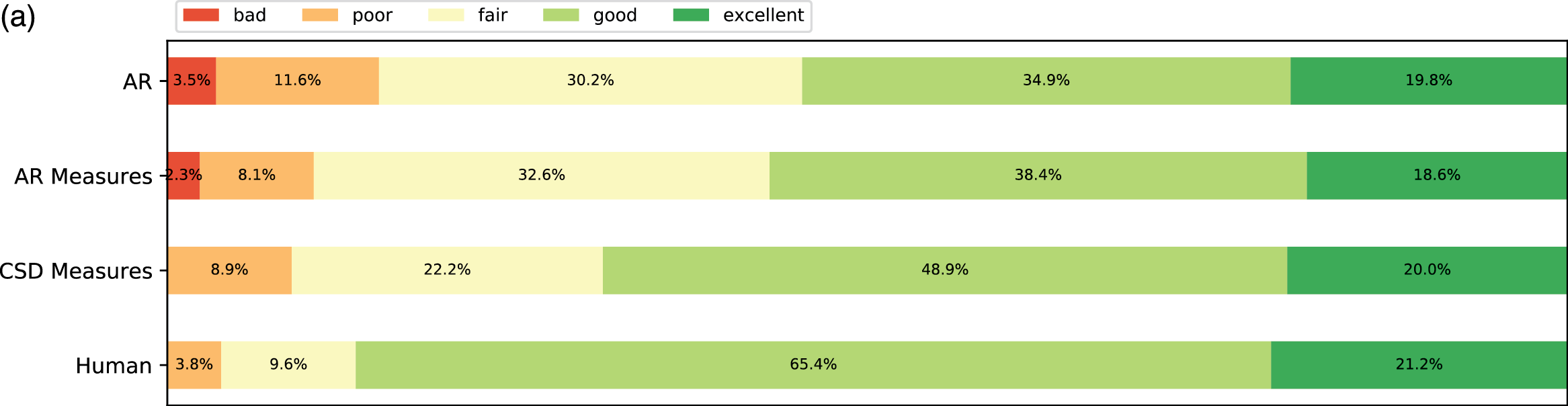
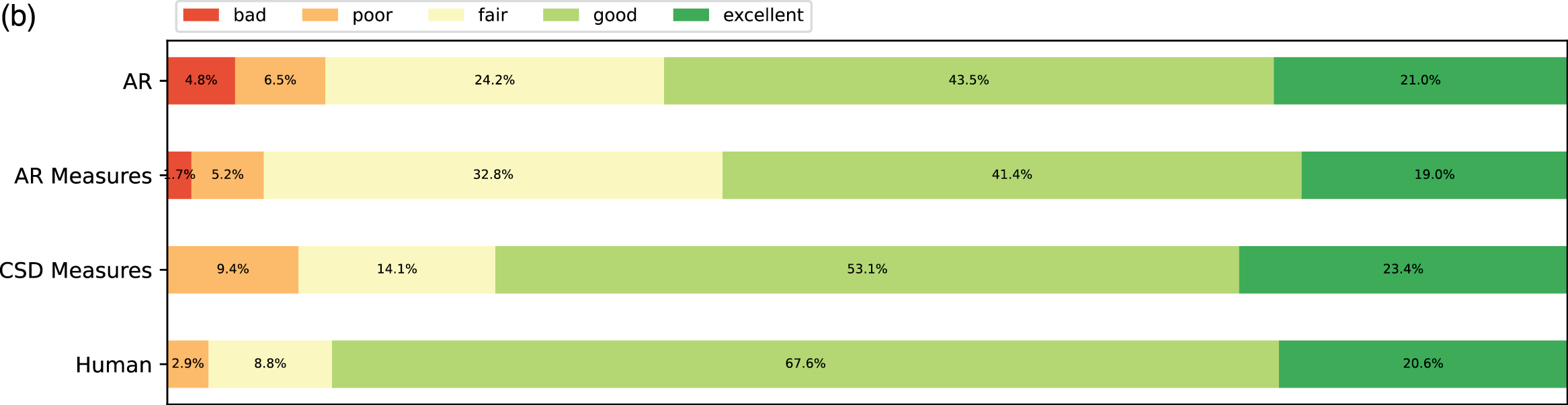
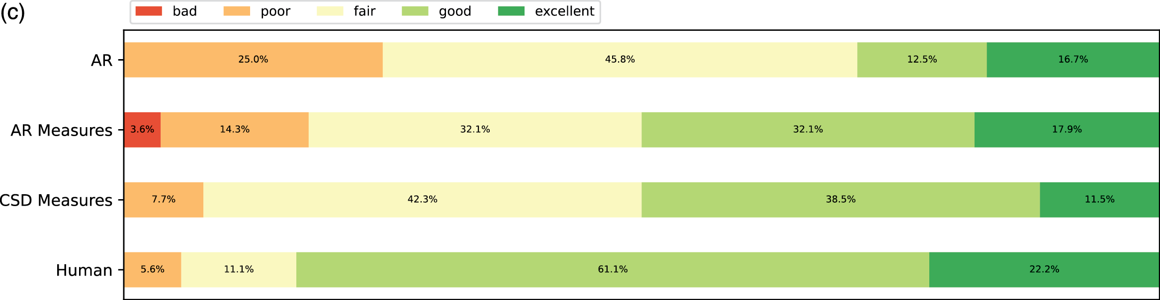
Figure 8
Subjective listening tests among different self‑reported expertise groups. (a) Overall ratings. (b) Overall ratings among those with the expertise “none/beginner”. (c) Overall ratings among those with the expertise “intermediate/experienced/expert”.
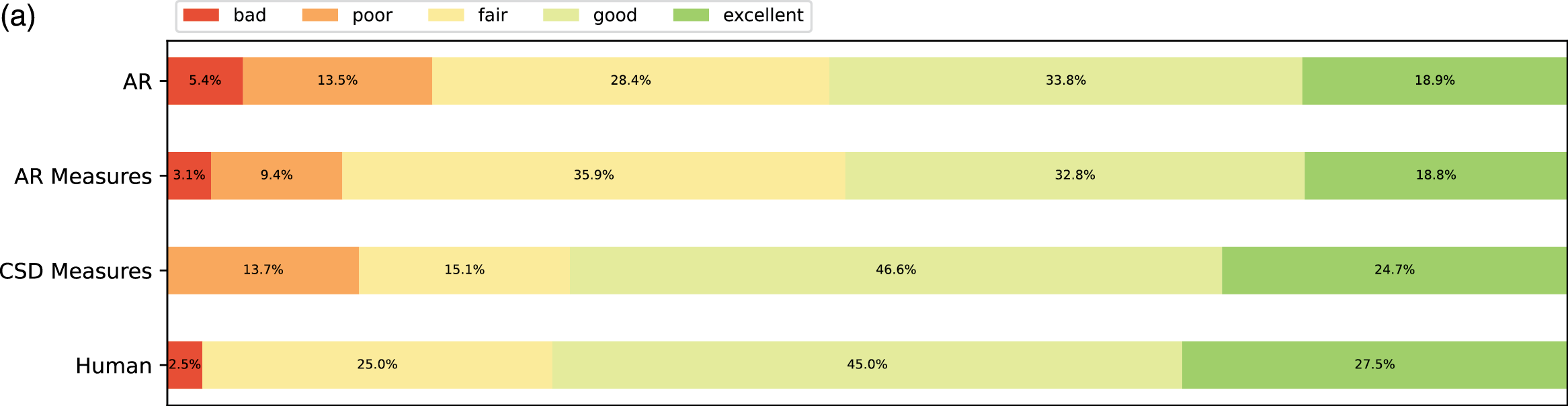
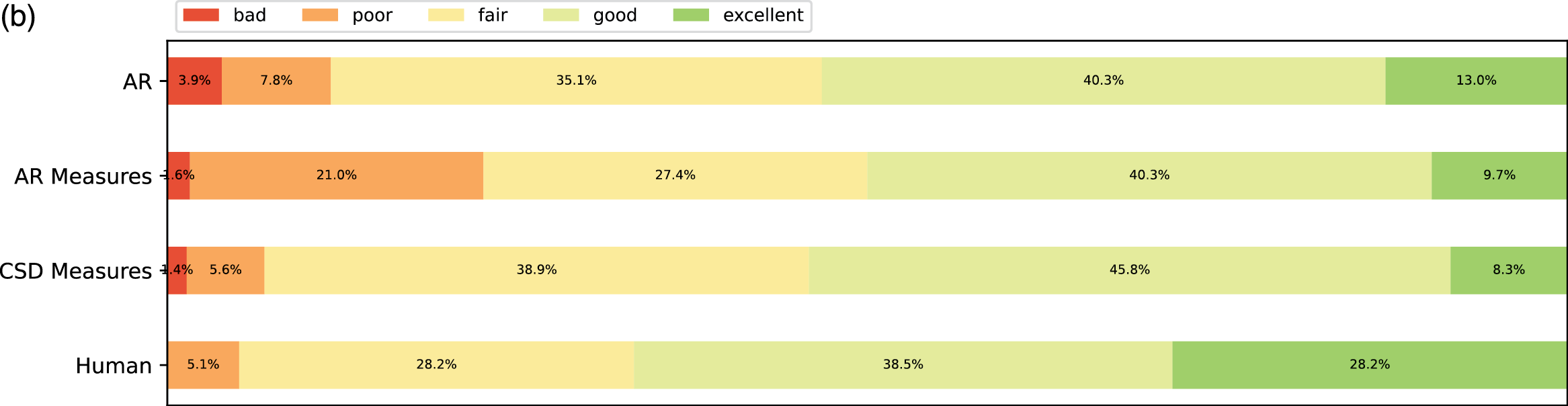
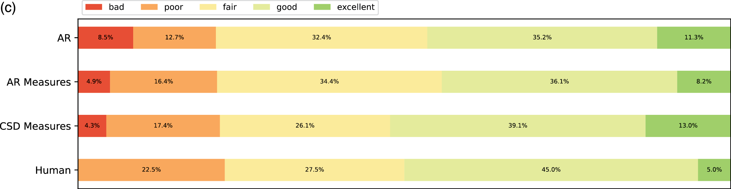
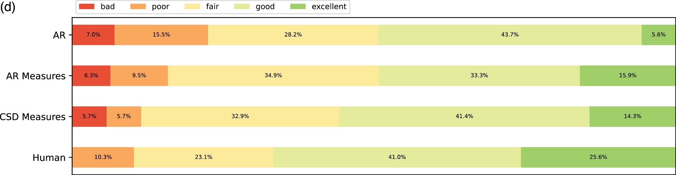
Figure 9
Subjective listening ratings along four aspects across all expertise groups. (a) Fluency. (b) Expressivity. (c) Novelty. (d) Organization.
From the ratings of all the expertise groups in Figure 9, AR Measure was slightly better than AR except for in expressivity and novelty. CSD was generally better than AR and AR Measure. To obtain more insight, we performed one‑sided Mann–Whitney rank tests to test whether a certain model had higher median ratings than another, as shown in Figure 10. From the pairwise comparison, the ‑values for each pair are generally not at a high significance level except for when it came to human versus others. However, on fluency CSD Measures out‑performed both AR and AR Measures at the significance level of 0.05, and on the overall rating, CSD Measures outperformed AR at the significance level of 0.1. The level of significance aligned with the comparison previously given in Figure 9.
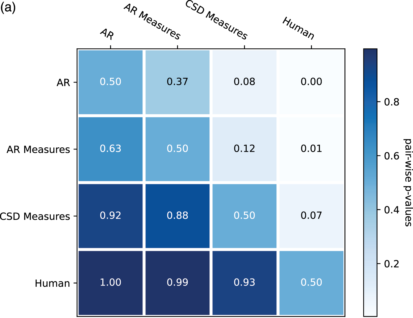
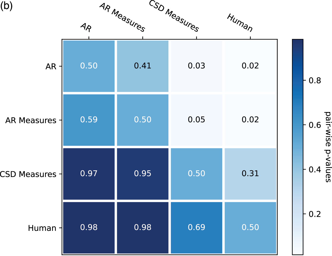
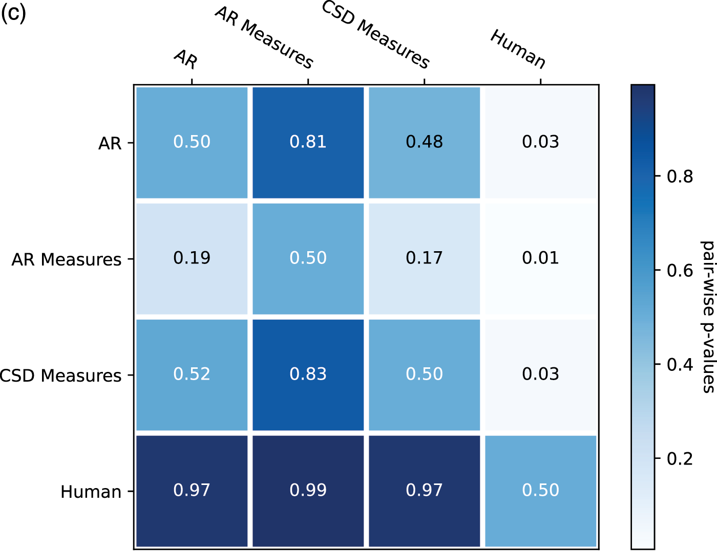
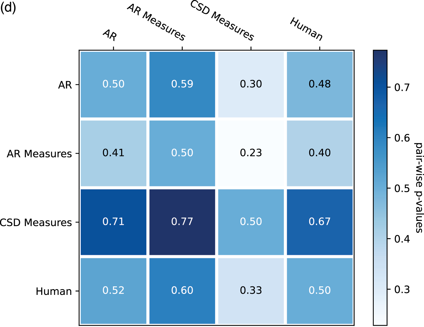
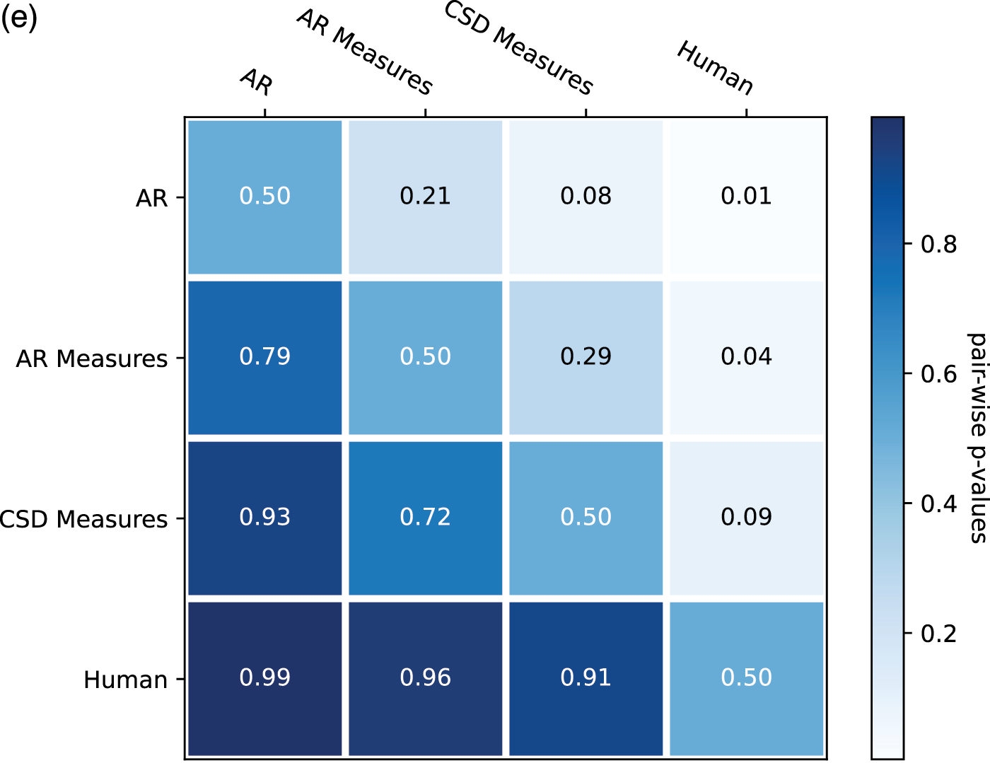
Figure 10
One‑sided Mann–Whitney rank test for the pairwise comparison of ratings: p‑value indicates the probability for the hypothesis that the median of population A (row) is larger than the median of population B (column). (a) Overall. (b) Fluency. (c) Expressivity. (d) Novelty. (e) Organization.
A unidimensional score derived from pairwise comparisons by the Bradley–Terry model using normalized U‑statistics3 from the Mann–Whitney test is shown in Table 3, which ranks all categories and is easier to interpret. As a reference group, human composers ranked the first for all rating categories except novelty, which is expected according to the definition. The autoregressive model with the measure model had a slightly higher overall/fluency/organization score but a slightly lower expressivity/novelty score than that without the measure model. This may be because the addition of the measure model to the generation process made the generated pieces more metrical (hence more fluent and organized) but reduced temporal fluctuations (hence less expressive or novel). Another possible reason is that using a measure as the basic generation unit reduces randomness at the note level, where more randomness may sound novel and expressive but less organized. The CSD model had higher ratings over all aspects than the AR models, as it learns to integrate information from arbitrary directions of generation. One observation is that it was difficult for AR models to end properly; the CSD model circumvented this by being informed when to end (the length of the piece in measures was given as a condition).
5.6 Human readability
Figure 11 gives one example of unconditional generation in regard to how the measure model can improve human readability of the generated music. The measure model, due to the design of independent measures, can recover from out‑of‑meter prediction errors (Figure 11, left), while such an error for a system without a measure model (Figure 11, right) results in a constant onset shift for all subsequent notes, which ruins the readability of the score. Additionally, because note spellings are built‑in features of the measure model, it also creates more readable note spellings (Figure 11, left).
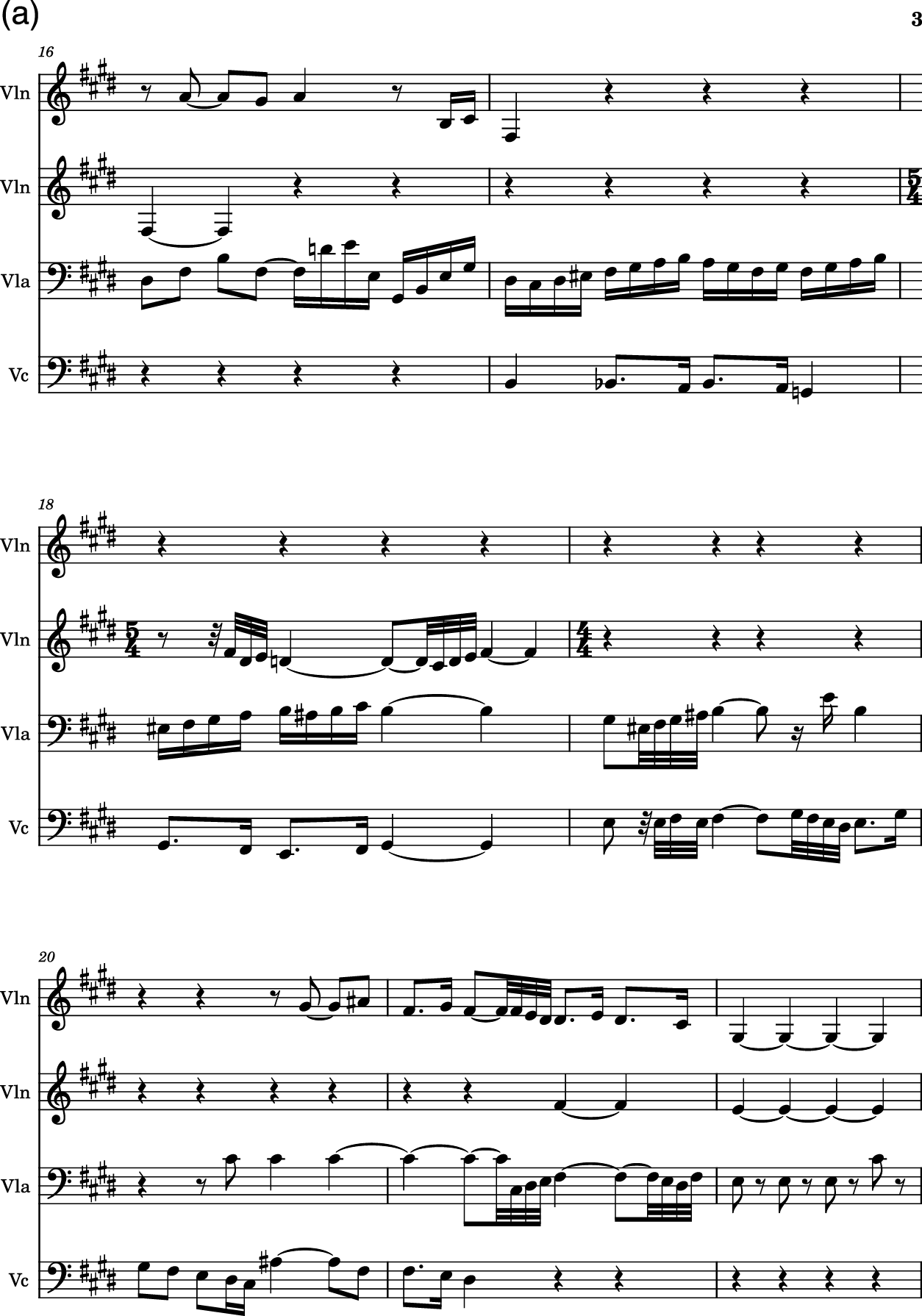
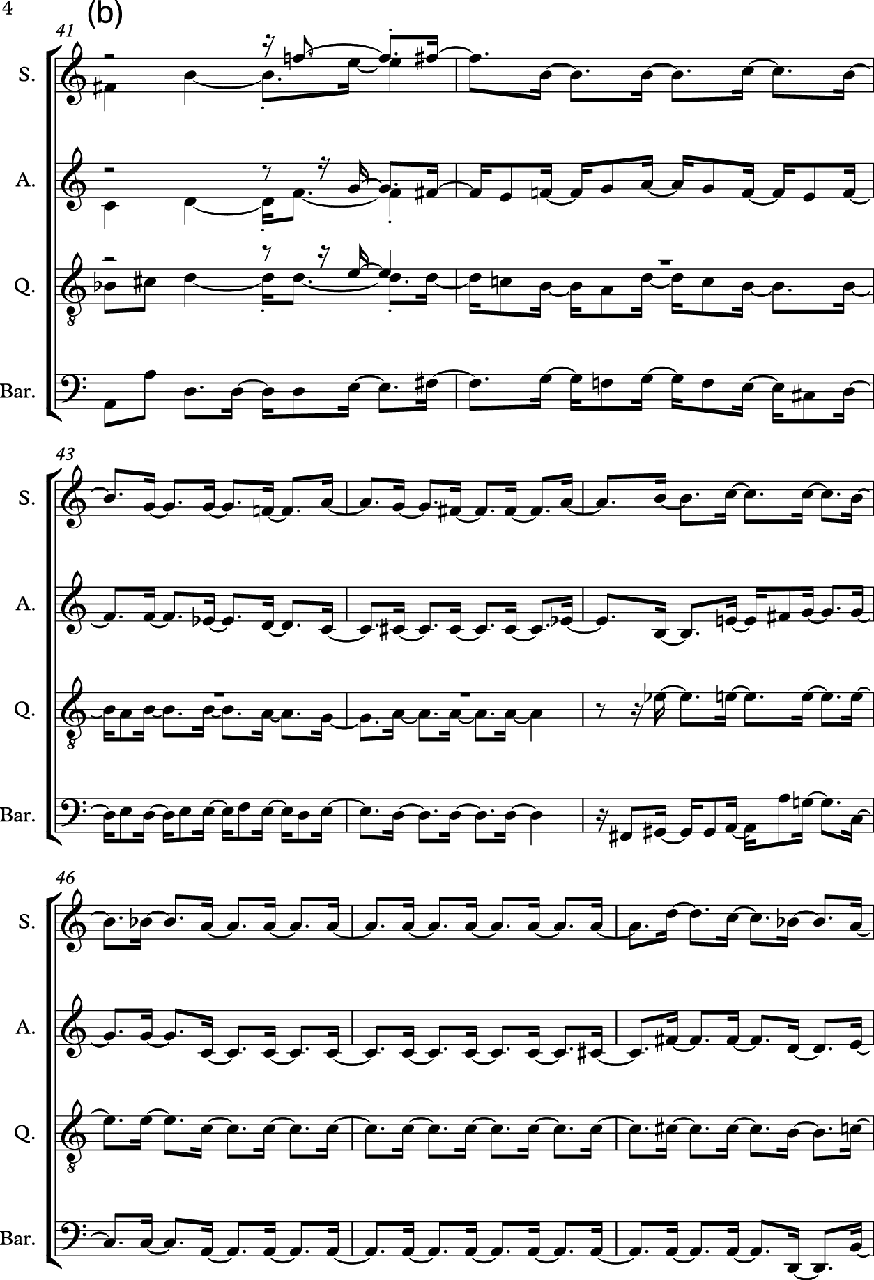
Figure 11
With the measure model, a beat sync error (left, m.18, second violin having an extra beat) can be recovered starting the next measure; without the measure model, this similar error (right, m.41, all parts having an extra 16th note) results in shifts in all subsequent note onset positions. (a) AR, with Measure Model. (b) AR, without Measure Model, output MIDI file imported by Sibelius.
5.7 Conditional generation
Appendix demonstrates the conditional generation capability of the proposed system by generating music with measures at arbitrary positions given as conditions. We created a string quartet arrangement for the melody of a Chinese folk song named Mo Li Hua. The melody was copied and transposed four times at several positions and parts as the given condition: violin 1 at m.1–m.14, violin 2 at m.15–m.28, cello at m.37–m.50, and viola at m.63–m.75. Our model was then used to perform inpainting. Copies of the original melody are marked with a circle at the note head. From the generated score, we can see that it automatically added accompaniments/counterpoints to the fixed melody line. Furthermore, between the appearances of the melody, it created sections that provided good contrast and smooth transitions. This example demonstrates the potential of using the proposed model for template‑based automatic arrangement.
6. Limitations and Future Work
From the attached example, we can clearly observe certain unstylistic elements, such as the harmonic cross‑relation of ♭B and ♮B followed by a dissonant harmonic interval of ♭E–F in the last measure of the first system on the second page. In the proposed model, unstylistic dissonances of this type typically arise from smooth voice leadings in different parts, violating the stylistic rules of the Baroque or Classical pieces the model was trained on. In addition, some of the notes are out of the register of the designated instruments. This exhibits the limited ability of the model to learn to satisfy both vertical and horizontal constraints if certain stylistic rules are viewed as a constraint satisfaction problem.
Limitations of the proposed approach include the requirement for well‑formed training data, which can be costly to obtain due to various issues with existing files freely available online. Another limitation is the granularity of a measure, which limits the ability to manipulate specific elements within a measure. Future work could explore the incorporation of more information across different levels to address this issue while maintaining efficiency and inductive bias.
7. Conclusions
In this work, we propose a framework that directly models the object hierarchy of the Western modern staff notation system to process and generate polyphonic music pieces originally written in modern staff notation. This was achieved by designing a structured encoder–decoder that represents the score as a grid of measure representations. We demonstrated how this framework can be used with a variety of paradigms for automatic music composition models, such as autoregressive models and conditionally specified distributions with masked conditional specifications. Subjective listening tests suggested that modeling polyphonic music as a grid of measures improves the fluency and organization of the generated pieces. Additionally, by enabling the paradigm of conditionally specified distributions, we demonstrated the capability of the proposed system to perform arbitrary conditioning.
Competing Interests
Zhiyao Duan is President of ISMIR. He is not involved in the running of TISMIR or its editorial board.
Additional File
The additional file for this article can be found as follows:
Notes
[1] One example of conditional distributions being inconsistent is that, for modeling two variables with conditional distributions and , there may not exist a , such that .