
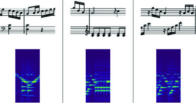
Figure 1
Audio-sheet music pairs presented to the network for embedding space learning.
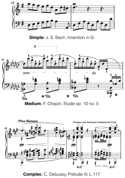
Figure 2
Example scores illustrating the range of music in MSMD, from simple to complex.
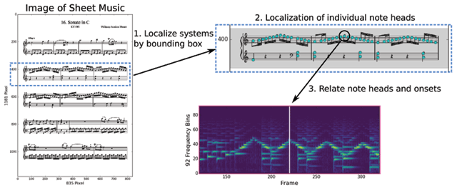
Figure 3
Core dataset workflow. For producing the alignment, it is necessary to “unroll” the score using individual staff systems, so that the ordering of noteheads in the score corresponds to the ordering of the notes in the MIDI file.
Table 1
MSMD statistics for the recommended train/test splits. Note that the numbers of noteheads, events, and aligned pairs do not match. This is because (a) not every notehead is supposed to be played, esp. tied notes; (b) some onsets do not get a notehead of their own, e.g. ornaments; (c) sometimes the alignment algorithm makes mistakes.
| Split Name | # Pieces/Aln. Pairs | Part | # Pieces | # Pages | # Noteheads | # Events | # Aln. Pairs |
|---|---|---|---|---|---|---|---|
| all | 479 / 344,742 | train | 360 | 970 | 316,038 | 310,377 | 308,761 |
| valid | 19 | 28 | 6,907 | 6,583 | 6,660 | ||
| test | 100 | 131 | 29,851 | 29,811 | 29,321 | ||
| bach-only | 173 / 108,316 | train | 100 | 251 | 77,834 | 75,283 | 74,769 |
| valid | 23 | 40 | 10,805 | 10,379 | 10,428 | ||
| test | 50 | 88 | 23,733 | 23,296 | 23,119 | ||
| bach-out | 479 / 344,742 | train | 281 | 725 | 235,590 | 233,041 | 231,617 |
| valid | 25 | 25 | 4,834 | 4,772 | 4,809 | ||
| test | 173 | 379 | 112,372 | 108,958 | 108,316 |
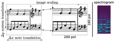
Figure 4
Overview of image augmentation strategies. The size of the sliding image window remains constant (160 × 200 pixels) but its content changes depending on the augmentations applied. The spectrogram remains the same for the augmented image versions.
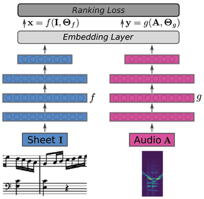
Figure 5
Architecture of correspondence learning network. The network is trained to optimize the similarity (in embedding space) between corresponding audio and sheet image snippets by minimizing a pair-wise ranking loss.
Table 2
Audio – sheet music model. BN: Batch Normalization (Ioffe and Szegedy, 2015), ELU: Exponential Linear Unit (Clevert et al., 2015), MP: Max Pooling, Conv (3, pad-1)–16: 3 × 3 convolution, 16 feature maps and padding 1.
| Sheet-Image 80 × 100 | Audio (Spectrogram) 92 × 42 |
|---|---|
| 2 × Conv(3, pad-1)-24 | 2 × Conv(3, pad-1)-24 |
| BN-ELU + MP(2) | BN-ELU + MP(2) |
| 2 × Conv(3, pad-1)-48 | 2 × Conv(3, pad-1)-48 |
| BN-ELU + MP(2) | BN-ELU + MP(2) |
| 2 × Conv(3, pad-1)-96 | 2 × Conv(3, pad-1)-96 |
| BN-ELU + MP(2) | BN-ELU + MP(2) |
| 2 × Conv(3, pad-1)-96 | 2 × Conv(3, pad-1)-96 |
| BN-ELU + MP(2) | BN-ELU + MP(2) |
| Conv(1, pad-0)-32-BN-LINEAR | Conv(1, pad-0)-32-BN-LINEAR |
| GlobalAveragePooling | GlobalAveragePooling |
| Embedding Layer + Ranking Loss | |

Figure 6
Sketch of sheet music-from-audio retrieval. The blue dots represent the embedded candidate sheet music snippets. The red dot is the embedding of an audio query. The larger blue dot highlights the closest sheet music snippet candidate selected as retrieval result.
Table 3
Snippet retrieval results. The table compares the influence of train/test splits and data augmentation on retrieval performance in both directions. For the audio augmentation experiments no sheet augmentation is applied and vice versa. none represents 1 sound font, with original tempo, and without sheet augmentation. We limit the number of retrieval candidates to 2000 for each of the splits to make the comparison across the different test sets fair.
| Audio-to-Sheet Retrieval | ||||||||||||
|---|---|---|---|---|---|---|---|---|---|---|---|---|
| bach-only | bach-out | all | ||||||||||
| Aug. | R@1 | R@25 | MRR | MR | R@1 | R@25 | MRR | MR | R@1 | R@25 | MRR | MR |
| none | 0.25 | 0.73 | 0.37 | 6 | 0.31 | 0.83 | 0.44 | 3 | 0.33 | 0.76 | 0.44 | 4 |
| sheet | 0.38 | 0.81 | 0.49 | 3 | 0.25 | 0.78 | 0.37 | 5 | 0.33 | 0.75 | 0.44 | 4 |
| audio | 0.48 | 0.87 | 0.59 | 2 | 0.38 | 0.83 | 0.50 | 2 | 0.46 | 0.82 | 0.57 | 2 |
| full | 0.52 | 0.87 | 0.62 | 1 | 0.46 | 0.86 | 0.57 | 2 | 0.50 | 0.83 | 0.60 | 2 |
| rand-bl | 0.00 | 0.01 | 0.0 | 1000 | 0.00 | 0.01 | 0.00 | 1000 | 0.00 | 0.01 | 0.00 | 1000 |
| Sheet-to-Audio Retrieval | ||||||||||||
| bach-only | bach-out | all | ||||||||||
| Aug. | R@1 | R@25 | MRR | MR | R@1 | R@25 | MRR | MR | R@1 | R@25 | MRR | MR |
| none | 0.34 | 0.81 | 0.46 | 3 | 0.35 | 0.83 | 0.48 | 3 | 0.39 | 0.80 | 0.51 | 2 |
| sheet | 0.45 | 0.85 | 0.57 | 2 | 0.28 | 0.80 | 0.42 | 4 | 0.40 | 0.79 | 0.52 | 2 |
| audio | 0.51 | 0.87 | 0.62 | 1 | 0.39 | 0.85 | 0.52 | 2 | 0.49 | 0.84 | 0.59 | 2 |
| full | 0.56 | 0.89 | 0.66 | 1 | 0.46 | 0.87 | 0.57 | 2 | 0.51 | 0.85 | 0.61 | 1 |
| rand-bl | 0.00 | 0.01 | 0.00 | 1000 | 0.00 | 0.01 | 0.00 | 1000 | 0.00 | 0.01 | 0.00 | 1000 |
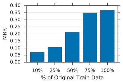
Figure 7
Influence of training set size on test set retrieval performance (MRR) evaluated on the bach-split in the no-augmentation setting.
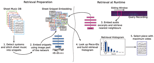
Figure 8
Piece retrieval concept from audio query. The entire pipeline consists of two stages: retrieval preparation and retrieval at runtime (best viewed in color, for details see Section 5).
Table 4
Piece and performance identification results on synthetic data for all three splits.
| Synthesized-to-Score | Score-to-Synthesized | |||||||||
|---|---|---|---|---|---|---|---|---|---|---|
| Train Split | # | Aug. | Rk@1 | Rk@5 | Rk@10 | >Rk10 | Rk@1 | Rk@5 | Rk@10 | >Rk10 |
| bach-only | 50 | none | 33 (0.66) | 46 (0.92) | 48 (0.96) | 2 (0.04) | 39 (0.78) | 48 (0.96) | 49 (0.98) | 1 (0.02) |
| full | 41 (0.82) | 49 (0.98) | 50 (1.00) | 0 (0.00) | 47 (0.94) | 50 (1.00) | 50 (1.00) | 0 (0.00) | ||
| bach-out | 173 | none | 125 (0.72) | 158 (0.91) | 163 (0.94) | 10 (0.06) | 145 (0.84) | 164 (0.95) | 166 (0.96) | 7 (0.04) |
| full | 143 (0.83) | 163 (0.94) | 167 (0.97) | 6 (0.03) | 149 (0.86) | 169 (0.98) | 172 (0.99) | 1 (0.01) | ||
| all | 100 | none | 67 (0.67) | 96 (0.96) | 98 (0.98) | 2 (0.02) | 94 (0.94) | 98 (0.98) | 99 (0.99) | 1 (0.01) |
| full | 82 (0.82) | 97 (0.97) | 99 (0.99) | 1 (0.01) | 92 (0.92) | 99 (0.99) | 100 (1.00) | 0 (0.00) | ||
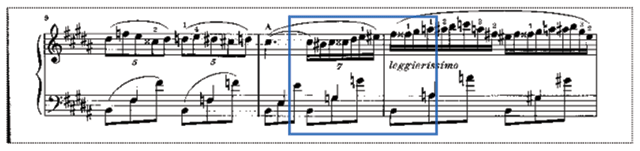
Figure 9
Exemplar staff line automatically extracted from a scanned score version of Chopin’s Nocturne Op. 9 No. 3 in B major (Henle Urtext Edition; reproduced with permission). The blue box indicates an example sheet snippet fed to the image part of the retrieval embedding network.
Table 5
Evaluation on real data: Piece retrieval results on scanned sheet music and recordings of real performances. The model used for retrieval is trained on the all-split with full data augmentation.
| Synthesized-to-Real-Score | Real-Score-to-Synthesized | ||||||||
|---|---|---|---|---|---|---|---|---|---|
| Composer | # | Rk@1 | Rk@5 | Rk@10 | >Rk10 | Rk@1 | Rk@5 | Rk@10 | >Rk10 |
| Mozart | 14 | 13 (0.93) | 14 (1.00) | 14 (1.00) | 0 (0.00) | 13 (0.93) | 14 (1.00) | 14 (1.00) | 0 (0.00) |
| Beethoven | 29 | 24 (0.83) | 27 (0.93) | 27 (0.93) | 2 (0.07) | 25 (0.86) | 27 (0.93) | 29 (1.00) | 0 (0.00) |
| Chopin | 150 | 127 (0.85) | 140 (0.93) | 145 (0.97) | 5 (0.03) | 112 (0.75) | 136 (0.91) | 142 (0.95) | 8 (0.05) |
| Performance-to-Real-Score | Real-Score-to-Performance | ||||||||
| Composer | # | Rk@1 | Rk@5 | Rk@10 | >Rk10 | Rk@1 | Rk@5 | Rk@10 | >Rk10 |
| Mozart | 14 | 5 (0.36) | 14 (1.00) | 14 (1.00) | 0 (0.00) | 12 (0.86) | 13 (0.93) | 13 (0.93) | 1 (0.07) |
| Beethoven | 29 | 16 (0.55) | 25 (0.86) | 27 (0.93) | 2 (0.07) | 20 (0.69) | 28 (0.97) | 28 (0.97) | 1 (0.03) |
| Chopin | 150 | 36 (0.24) | 72 (0.48) | 91 (0.61) | 59 (0.39) | 58 (0.39) | 94 (0.63) | 111 (0.74) | 39 (0.26) |