
Table 1
Entries and final places for the AI Song Contest 2020.
| Place | Country | Team | Song |
|---|---|---|---|
| 1 | Australia | Uncanny Valley | Beautiful the World |
| 2 | Germany | Dadabots × Portrait XO | I’ll Marry You Punk Come |
| 3 | The Netherlands | Can AI Kick It | Abbus |
| 4 | France | Algomus & Friends | I Keep Counting |
| 5 | The Netherlands | COMPUTD/Shuman & Angel-Eye | I Write a Song |
| 6 | United Kingdom | Brentry | Hope Rose High |
| 7 | Belgium | Polaris | Princess |
| 8 | Belgium | Beatroots | Violent Delights Have Violent Ends |
| 9 | France | DataDada | Je secoue le monde |
| 10 | Sweden | KTH/KMH + Doremir | Come To Ge Ther |
| 11 | Germany | OVGneUrovision | Traveller in Time |
| 12 | Germany | Ligatur | Offshore in Deep Water |
| 13 | Switzerland | New Piano | Painful Words |

Figure 1
Development of voters’ average scores over time and final jury scores. The voting sites were open from 10 April 2020 through 10 May 2020; the jury scores and final results were announced in a live broadcast on 12 May 2020. Each song’s final score was the sum of its average voter score and its score from the jury.2 The jury favourite, ‘I’ll Marry You Punk Come’, was a notable area of disagreement between the jury and the voters.

Figure 2
Distribution of votes across teams and voters’ frequency of voting. Most voters voted either for all thirteen teams (11%) or just one (67%). One-time voters were distributed quite unevenly across the entries and constituted 45% of all votes for the extreme case of ‘Beautiful the World’.
Table 2
Prior and hyper-prior distributions for the hierarchical Rasch models. The choices are weakly informative with regularising tails.
| Parameter | Description |
|---|---|
| Priors | |
| γn ~ N(µγ, σγ) | Logit three-inflation |
| θn ~ N(0, σθ) | Song quality |
| δi ~ N(µδ, σδ) | Criterion difficulty |
| λj ~ N(0, σλ) | Voter or judge severity |
| τk ~ N(0, στ) | Rating-threshold offset |
| ζik ~ N(0, σζ) | Partial-credit interaction |
| Hyper-Priors | |
| µγ ~ N(0, 1) | Mean logit three-inflation |
| µδ ~ N(0, 1) | Intercept |
| σγ ~ N+(0, 1) | SD logit three-inflation |
| σθ ~ N+(0, 1) | SD song quality |
| σδ ~ N+(0, 1) | SD criterion difficulty |
| σλ ~ N+(0, 1) | SD voter or judge severity |
| στ ~ N+(0, 1) | SD threshold offset |
| σζ ~ N+(0, 1) | SD partial-credit interaction |
Table 3
Approximate information criteria under leave-one-song-out cross-validation (LOO-IC; lower is better). The observations are weighted such that voters’ ratings (on scales of 0 to 3) and the judges’ ratings (on scales of 0 to 2) contribute equally to the likelihood. The intercept-only model serves as a simple baseline. Leave-one-song-out cross-validation is conservative, and only three models outperform the baseline (in italics and bold); the many-facet partial-credit model without three inflation performs best.
| Model | Facets | Three Inflation | Parameter Count | LOO-IC |
|---|---|---|---|---|
| Intercept Only | Single | No | 15 | 144 944 |
| Rating Scale | Single | No | 30 | 147 378 |
| Rating Scale | Single | Yes | 45 | 150 455 |
| Partial Credit | Single | No | 49 | 153 181 |
| Partial Credit | Single | Yes | 64 | 144 044 |
| Rating Scale | Many | No | 3860 | 145 056 |
| Rating Scale | Many | Yes | 3875 | 144 796 |
| Partial Credit | Many | No | 3879 | 143 402 |
| Partial Credit | Many | Yes | 3894 | 151 248 |

Figure 3
Rasch calibrations for the AI Song Contest evaluation scheme. (A–C) present kernel density estimates of the calibrations for song quality, voters’ criterion difficulty, and the jury’s criterion difficulty, all on a standard T scale (M = 50, SD = 10). Plot labels are followed by point estimates of the calibrations (posterior medians) as well as the reliability coefficients for these estimates (in parentheses). The density estimates are marked with their medians and the 2.5% and 97.5% quantiles (i.e., a 95% credible interval). For the rating criteria, the densities for each step of the scale are shown individually. (D) presents density estimates for the severities of the voters who voted for each entry, coloured by tail probability (dark blue for the median ranging to yellow at the extrema of the distributions). ‘Groupies’ are prominently visible, especially for ‘Beautiful the World’ and ‘I Write a Song’. (E) is the same visualisation but excluding all voters who gave perfect scores or perfect zeros. The groupie effect disappears.
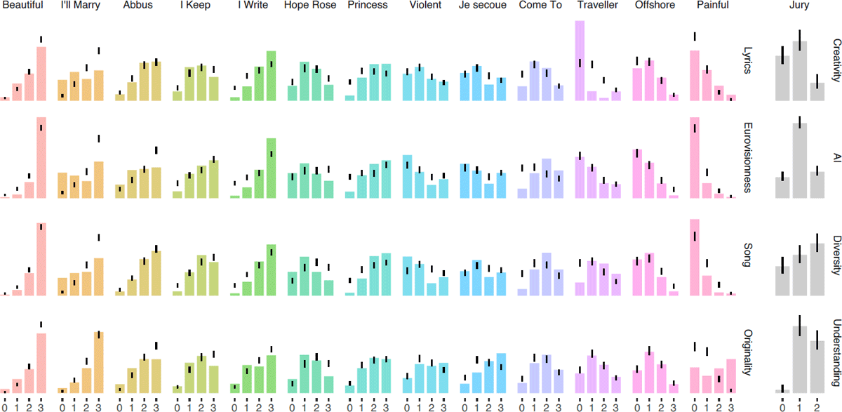
Figure 4
Posterior predictive checks on the distribution of ratings. Observed data appear as histograms; black lines cover 95% of the corresponding histograms from 2000 simulated data sets using parameter values sampled from the posterior distribution. For the voters, we provide an analysis per song, but in order to preserve the anonymity of judges, we only provide aggregated data for the jury. In general, the model seems to be well calibrated, but there are a few notable miscalibrations for ‘I’ll Marry You Punk Come’ and ‘Traveller in Time’.