
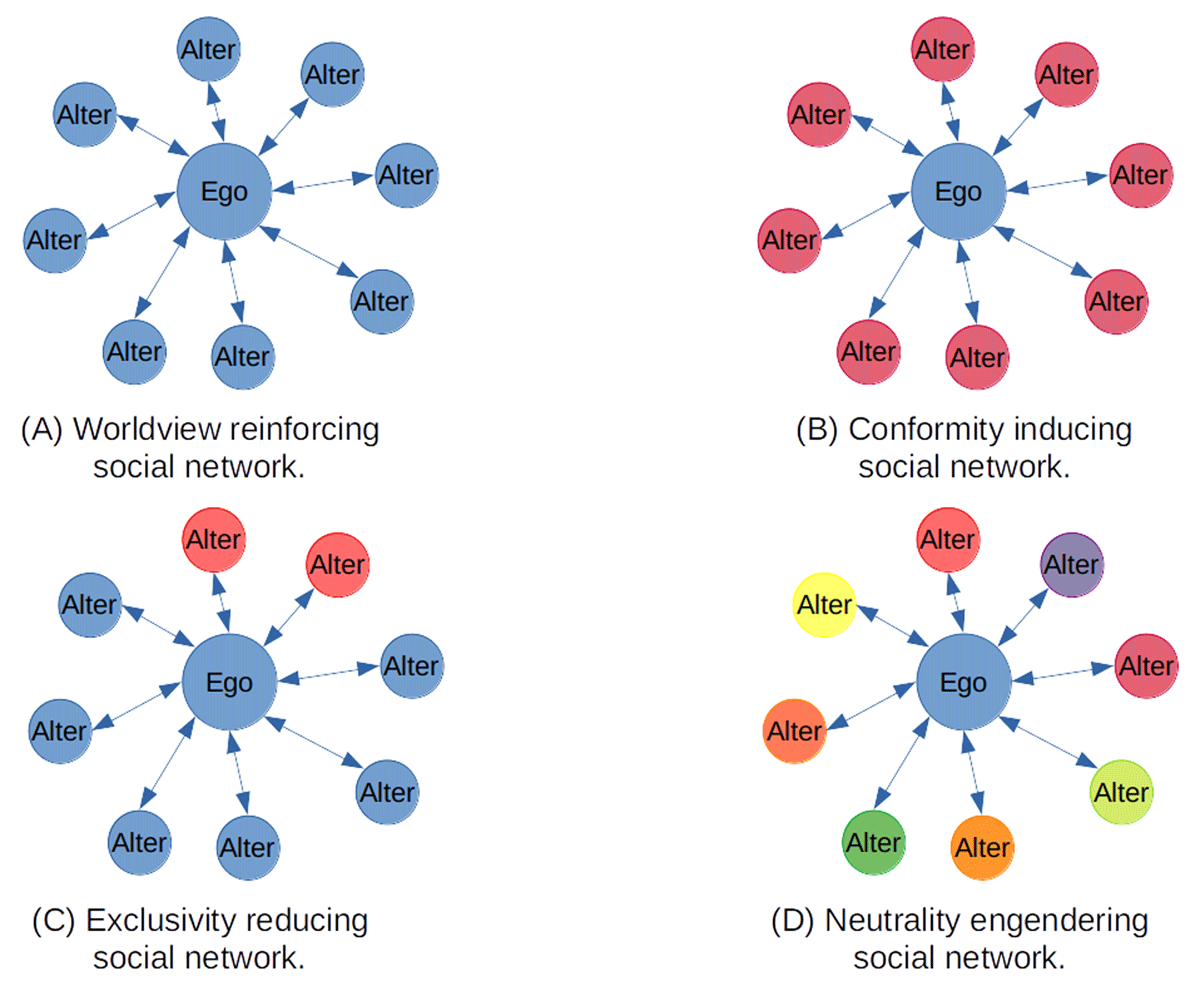
Figure 1
Social network variations and their relation to worldview change.
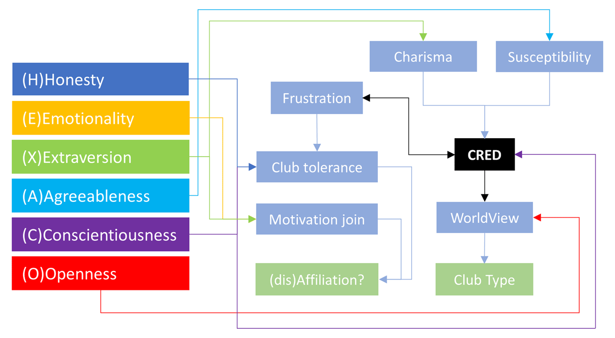
Figure 2
Relation between HEXACO personality factors, CRED displays, WV values, and (dis)affiliation with/from religious clubs.
Openness influences initial WV value of the agent; agreeableness influences susceptibility; extraversion influences charisma; honesty and conscientiousness influence club tolerance (CT); emotionality and extraversion influence motivation to join a club (MJC); and conscientiousness and frustration influence CRED consistency. Observing others display CREDs may change/reinforce agent’s WV values and may increase/decrease their frustration. High frustration may lead to club disaffiliation and/or reaffiliation via CT and MJC.
Table 1
Average WV value and percentage of affiliation of the three societies selected for this study.
| Society | |||
|---|---|---|---|
| H-H | L-M | L-L | |
| Average WV value of the society at year 30 | 0.91 | 0.34 | 0.26 |
| % of agents affiliated with a club at year 30 | 91% | 52% | 14% |
Table 2
Data collected for each agent every simulation year.
| Agent’s variable | Description | Type |
|---|---|---|
| Age | Age of the agent | Numeric |
| Generation | Initial population is generation 1; thereafter, as agents are born, they inherit their parents generation + 1. | Categorical |
| Education | Number of years agent was/is being educated | Numeric |
| Occupation Status | Student, employed or unemployed | Categorical |
| Gender | Male or female | Categorical |
| Group | Minority or Majority | Categorical |
| Income | Income of the agent | Numeric |
| Income class | Low, medium-low, medium, medium-high, high | Categorical |
| Marital Status | Single, married or widowed | Categorical |
| Number of Children | 0, 1, 2, 3, 4, or 5 | Categorical |
| Agreeableness | Value of the agent’s personality trait | Numeric |
| Openness | Value of the agent’s personality trait | Numeric |
| Susceptibility | Value of the agent’s personality trait | Numeric |
| Worldview | Value of agent’s worldview | Numeric |
| Hypocrisy Threshold | Value of the agent’s personality trait | Numeric |
| Motivation to Join | Value of the agent’s personality trait | Numeric |
| Frustration | Value of the agent’s personality trait | Numeric |
| Ave WV Family | Average WV Family | Numeric |
| Ave WV OFSN | Average WV of offline social network | Numeric |
| Ave WV Club | Average WV of club | Numeric |
| Existential Security effect | Value of the agent’s existential security | Numeric |
| Homogeneity score | Value of the agent’s homogeneity score | Numeric |
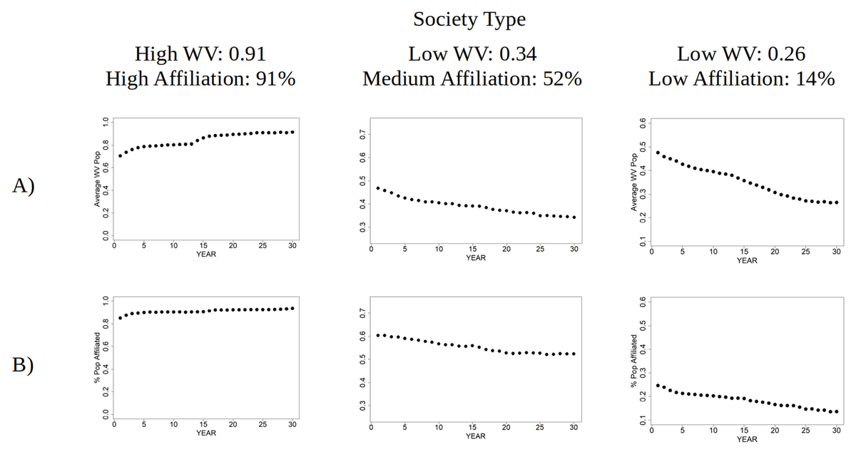
Figure 3
Evolution of A) WV value of the population (y-axis) and B) percentage of agents affiliated (y-axis) during simulation years (x-axis) and type of society.
Table 3
Logistic regression model predicting affiliation (1) or no affiliation (0) with a religious club among agents of the society with high values of WV and high percentage of affiliation.
| Estimate | Std Error | z value | P-value | |
|---|---|---|---|---|
| (Intercept) | –39.83 | 8.53 | –4.67 | 0.000 |
| Marital Status: SINGLE | –1.53 | 0.68 | –2.27 | 0.023 |
| Marital Status: WIDOWED | 1.25 | 1.08 | 1.16 | 0.247 |
| Openness | 4.53 | 2.04 | 2.22 | 0.027 |
| Motivation to join | 6.07 | 7.38 | 0.82 | 0.411 |
| Homogeneity score | 39.35 | 4.92 | 7.99 | 0.000 |
| Income class: LOWEST CLASS | 0.76 | 1.00 | 0.77 | 0.445 |
| Income class: MIDDLE CLASS | 2.40 | 1.07 | 2.26 | 0.024 |
| Income class: MIDDLE HIGH CLASS | 2.21 | 1.31 | 1.69 | 0.091 |
| Income class: MIDDLE LOW CLASS | 0.75 | 1.17 | 0.64 | 0.520 |
[i] Nagelkerke pseudo R2 index: 0.89.
Reference category for marital status is MARRIED and for income class HIGHEST CLASS.
In bold: significant predictors.
Table 4
Logistic regression model predicting affiliation (1) or not affiliation (0) with a religious club among agents of the society with low values of WV and low percentage of affiliation.
| Estimate | Std Error | z value | P-value | |
|---|---|---|---|---|
| (Intercept) | –1.59 | 2.98 | –0.53 | 0.593 |
| Motivation to join | 9.73 | 3.01 | 3.23 | 0.001 |
| Frustration | 2.93 | 0.47 | 6.22 | 0.000 |
| Existential Security effect | –2.25 | 0.97 | –2.33 | 0.020 |
| Homogeneity score | –9.80 | 1.06 | –9.26 | <0.001 |
| Income class: LOWEST CLASS | 0.22 | 0.51 | 0.43 | 0.664 |
| Income class: MIDDLE CLASS | 0.35 | 0.40 | 0.89 | 0.376 |
| Income class: MIDDLE HIGH CLASS | 0.29 | 0.47 | 0.61 | 0.541 |
| Income class: MIDDLE LOW CLASS | 0.29 | 0.55 | 0.53 | 0.594 |
[i] Nagelkerke pseudo R2 index: 0.26.
Reference category for income class HIGHEST CLASS.
In bold: significant predictors.
Table 5
Logistic regression model predicting affiliation (1) or not affiliation (0) with a religious club among agents of the society with low values of WV and medium percentage of affiliation.
| Estimate | Std Error | z value | P-value | |
|---|---|---|---|---|
| (Intercept) | 4.83 | 0.64 | 7.51 | <0.001 |
| Motivation to join | 1.90 | 0.58 | 3.26 | 0.001 |
| Frustration | 4.93 | 0.54 | 9.20 | <0.001 |
| Homogeneity score | –7.67 | 0.56 | –13.77 | <0.001 |
| Income class: LOWEST CLASS | –0.58 | 0.22 | –2.60 | 0.009 |
| Income class: MIDDLE CLASS | –0.34 | 0.21 | –1.67 | 0.095 |
| Income class: MIDDLE HIGH CLASS | –0.20 | 0.26 | –0.79 | 0.429 |
| Income class: MIDDLE LOW CLASS | –0.16 | 0.25 | –0.62 | 0.532 |
[i] Nagelkerke pseudo R2 index: 0.26.
Reference category for income class HIGHEST CLASS.
In bold: significant predictors.
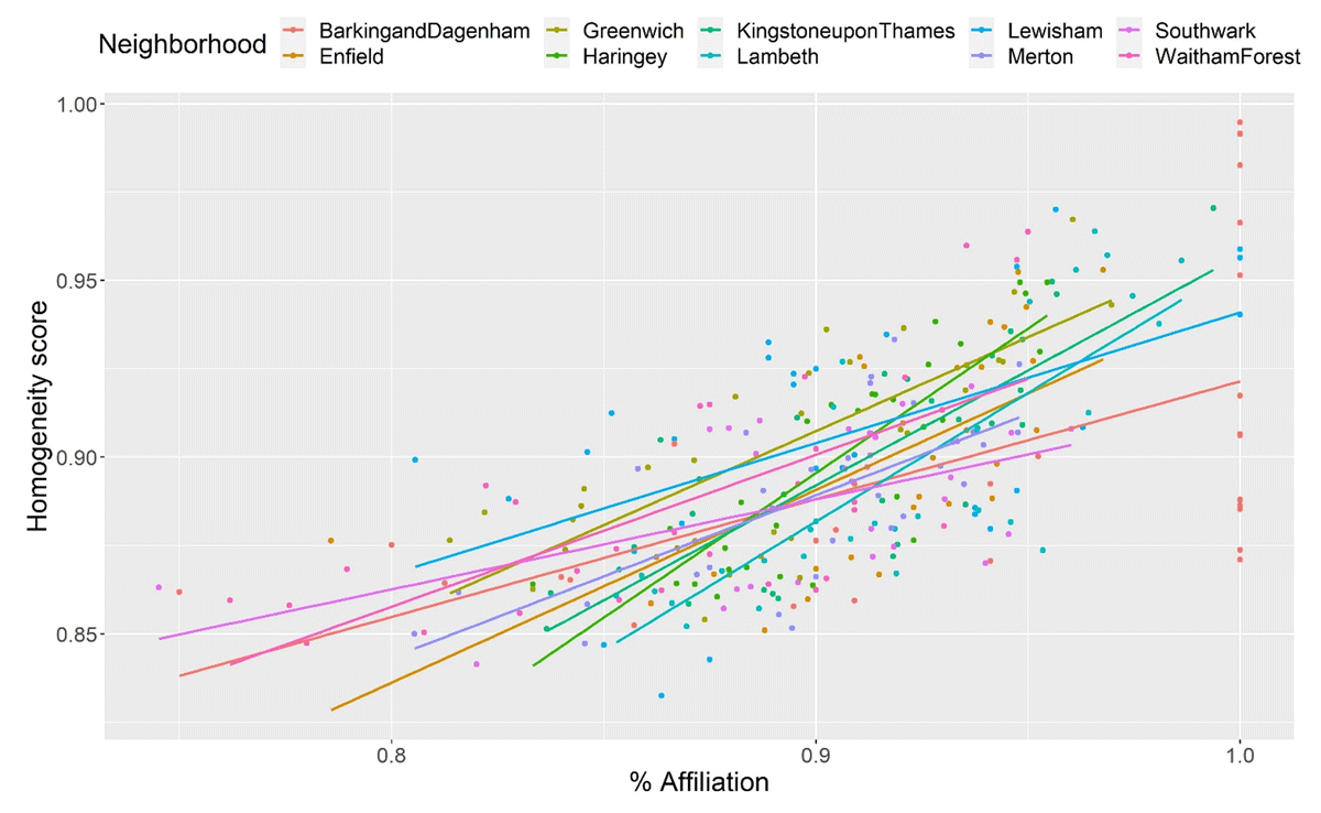
Figure 4
Relationship between percentage of affiliation and homogeneity score at the neighborhood level in the society with high WV and percentage of affiliation values.
Table 6
Generalized linear mixed models for A) society with high WV and affiliation, B) society with low WV and affiliation, and C) society with low WV and medium affiliation.
| A) Society with high WV and high percentage of affiliation values | ||||
|---|---|---|---|---|
| Fixed effects | Coefficient | Std Error | t value | p-value |
| (Intercept) | –0.13 | 0.09 | –1.47 | 0.142 |
| Year | 0.00 | 0.00 | –2.46 | 0.014 |
| Homogeneity score | 1.17 | 0.10 | 11.20 | <0.001 |
| Random effect | Variance | Std. Error | ||
| Neighborhood | 0.0002 | 0.015 | ||
| Residual | 0.0012 | 0.034 | ||
| B) Society with low WV and low percentage of affiliation values | ||||
| Fixed effects | Coefficient | Std Error | t value | p-value |
| (Intercept) | 1.27 | 0.22 | 5.79 | <0.001 |
| Year | –0.01 | 0.00 | –7.25 | <0.001 |
| Homogeneity score | –1.15 | 0.25 | –4.67 | <0.001 |
| Random effect | Variance | Std. Error | ||
| Neighborhood | 0.0007 | 0.027 | ||
| Residual | 0.0055 | 0.074 | ||
| C) Society with low WV and medium percentage of affiliation values | ||||
| Fixed effects | Coefficient | Std Error | t value | p-value |
| (Intercept) | 0.773 | 0.183 | 4.221 | <0.001 |
| Year | –0.001 | 0.000 | –2.477 | 0.014 |
| Homogeneity score | –0.244 | 0.217 | –1.126 | 0.261 |
| Random effect | Variance | Std. Error | ||
| Neighborhood | 0.002 | 0.044 | ||
| Residual | 0.007 | 0.086 | ||
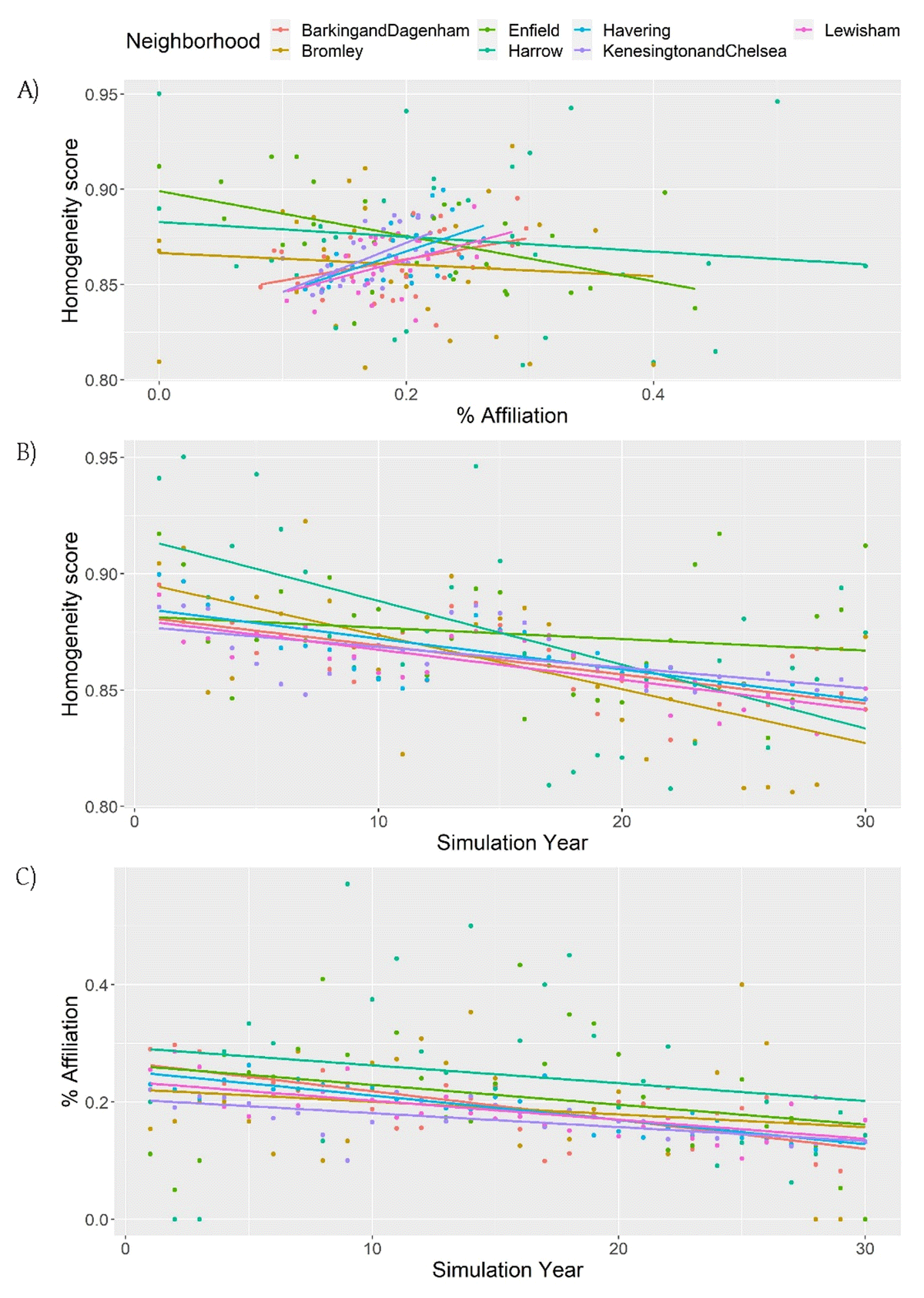
Figure 5
Relationship between A) percentage of affiliation and homogeneity score, B) Homogeneity score and simulation year, C) percentage of affiliation and simulation year at the neighborhood level in the society with low WV and percentage of affiliation values.
Table 7
Pearson correlations and linear model predicting percentage of affiliation at the neighborhood level in the society with low values of WV and low percentage of affiliation.
| Neighborhood | Pearson correlation coefficient: | D) LM: Aff ~ Year + Hom | |||
|---|---|---|---|---|---|
| A) Hom Vs Year | B) Aff Vs Year | C) Aff Vs Hom | Estimate Year | Estimate Hom | |
| 1) Barking and Dagenham | –0.670*** | –0.741*** | 0.399* | –0.006*** | –0.635NS |
| 2) Bromley | –0.630*** | –0.194NS | –0.093NS | –0.005NS | –1.069NS |
| 3) Enfield | –0.177NS | –0.282NS | –0.514** | –0.005* | –2.525*** |
| 4) Harrow | –0.578*** | –0.191NS | –0.131NS | –0.006NS | –1.219NS |
| 5) Havering | –0.783*** | –0.875*** | 0.607*** | –0.005*** | –0.567NS |
| 6) Kensington and Chelsea | –0.586*** | –0.657*** | 0.616*** | 0.001* | 0.837* |
| 7) Lewisham | –0.798*** | –0.687*** | 0.495*** | –0.004** | –0.356NS |
[i] Hom = homogeneity score; Aff = percentage of affiliation; Year = simulation year; LM = linear model. Significance values: NS = not significant, * <0.05; ** <0.01; *** <0.001.
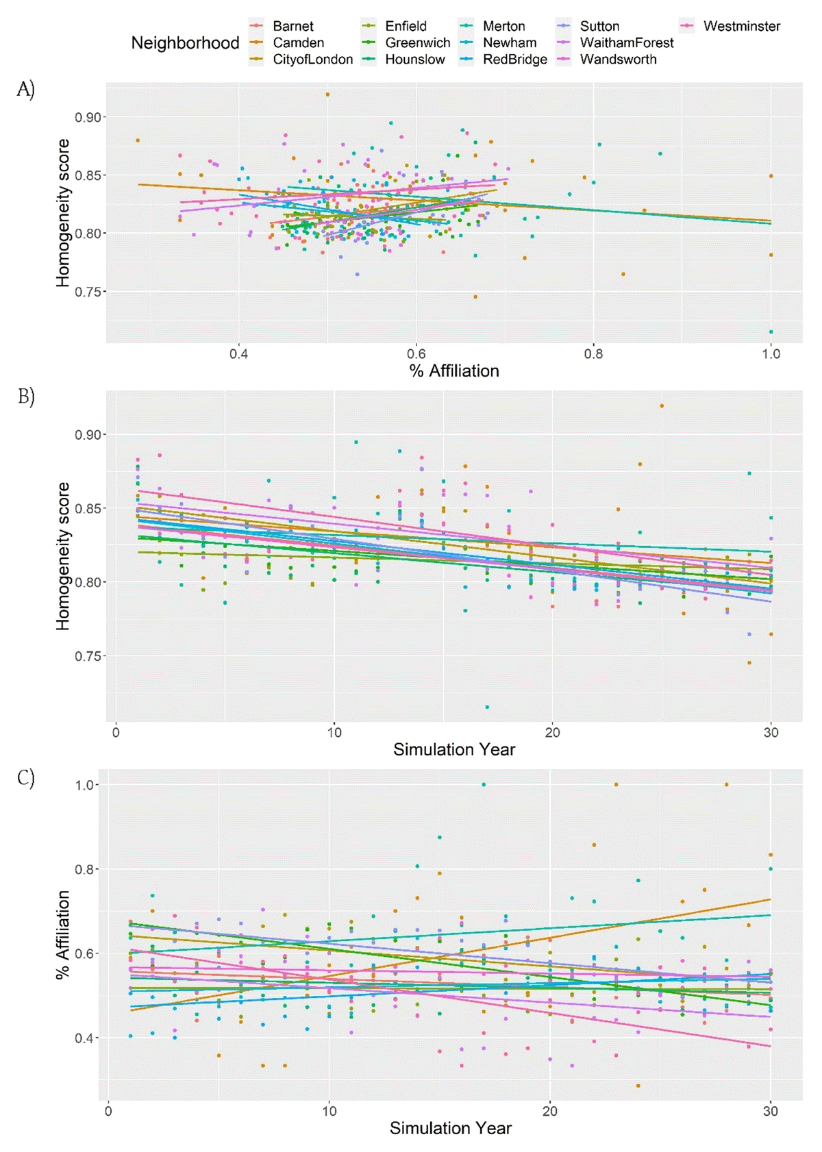
Figure 6
Relationship between A) percentage of affiliation and homogeneity score, B) Homogeneity score and simulation year, C) percentage of affiliation and simulation year at the neighborhood level in the society with low WV and medium percentage of affiliation values.
Table 8
Pearson correlations and linear model predicting percentage of affiliation at the neighborhood level in the society with low values of WV and medium percentage of affiliation.
| Neighborhood | Pearson correlation coefficient: | D) LM: Aff ~ Year + Hom | |||
|---|---|---|---|---|---|
| A) Hom Vs Year | B) Aff Vs Year | C) Aff Vs Hom | Estimate Year | Estimate Hom | |
| Barnet | –0.65*** | –0.28NS | 0.24NS | –0.001NS | 0.28NS |
| City of London | –0.82*** | –0.58*** | 0.36* | –0.005** | –0.99NS |
| Enfield | –0.25NS | –0.02NS | –0.09NS | –0.000NS | –0.37NS |
| Greenwich | –0.519** | –0.815*** | 0.382* | –0.007*** | –0.25NS |
| Hounslow | –0.578** | –0.208NS | 0.328NS | –0.000NS | 0.81NS |
| New Ham | –0.819*** | 0.144NS | –0.265NS | –0.002NS | –1.54NS |
| Red Bridge | –0.817*** | 0.431* | –0.399* | 0.002NS | –0.438 |
| Sutton | –0.813*** | –0.699*** | 0.497** | –0.006*** | –0.53NS |
| Waitham Forest | –0.506*** | –0.332NS | 0.26NS | –0.003NS | 0.42NS |
| Wandsworth | –0.727*** | –0.175NS | 0.234NS | 0.000NS | 0.49NS |
| Westminster | –0.665*** | –0.686*** | 0.163NS | –0.011*** | –2.04** |
[i] Hom = homogeneity score; Aff = percentage of affiliation; Year = simulation year; LM = linear model. Significance values: NS = not significant, * <0.05; ** <0.01; *** <0.001.