
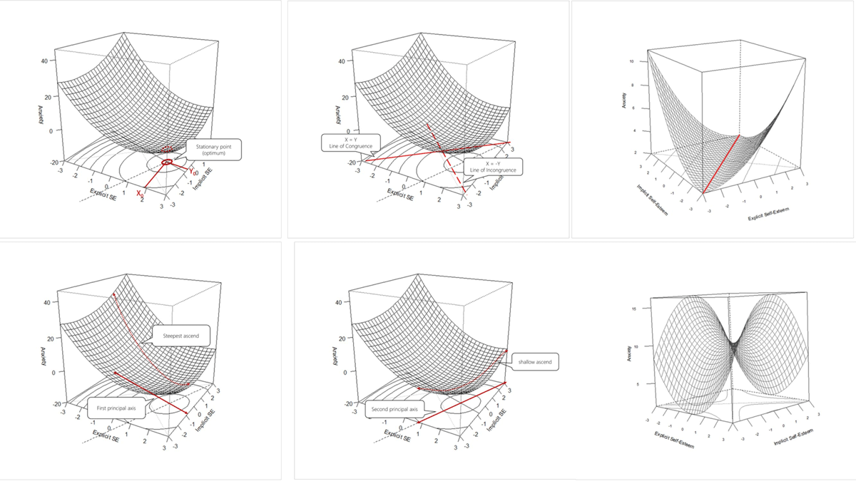
Figure 1
Six visualizations to explain RSA graphically.
Table 1
Means, standard deviations, and correlations with confidence intervals of all research variables after data imputation, N = 135.
| VARIABLE | M | SD | 1 | 2 | 3 | 4 | 5 | 6 |
|---|---|---|---|---|---|---|---|---|
| 1. Depression | 4.22 | 3.77 | ||||||
| 2. Anxiety | 5.48 | 5.02 | .78** [.71, .84] | |||||
| 3. Aggression | 2.79 | 22.42 | .48** [.34, .60] | .57** [.45, .68] | ||||
| 4. Explicit SE | 21.20 | 5.06 | –.61** [–.71, –.49] | –.57** [–.68, –.45] | –.24** [–.39, –.07] | |||
| 5. Implicit SE | 0.28 | 00.37 | .02 [–.15, .19] | .09 [–.08, .26] | –.05 [–.22, .12] | .01 [–.16, .18] | ||
| 6. contDif | –0.00 | 10.41 | .45** [.30, .57] | .47** [.33, .59] | .13 [–.04, .29] | –.70** [–.78, –.61] | .70** [.61, .78] | |
| 7. CreemersDif | 1.11 | 00.87 | .26** [.09, .41] | .29** [.13, .44] | .18* [.01, .34] | –.15 [–.31, .02] | –.07 [–.24, .10] | .05 [–.12, .22] |
[i] Note: M and SD are used to represent mean and standard deviation, respectively.
Values in square brackets indicate the 95% confidence interval for each correlation. The confidence interval is a plausible range of population correlations that could have caused the sample correlation (Cumming, 2014).
* Indicates p < .05. ** Indicates p < .01.
Table 2
Frequency counts for the two categorical difference score variables: categorical difference (congruent, damaged and fragile SE), and the dummy variable used in Creemer’s method (damaged and fragile). N = 135.
| CONGRUENT | DAMAGED | FRAGILE | |
|---|---|---|---|
| Categorical | 39 | 47 | 49 |
| Creemer’s dummy | NA | 67 | 68 |
Table 3
The continuous difference score (z-implicit – z-explicit)and it quadratic term as orthogonal predictors of standardized depression, anxiety, and aggression. In block one the main effect is modelled, in the second block the quadratic term is added.
| DEPRESSION | ANXIETY | AGGRESSION | ||||
|---|---|---|---|---|---|---|
| (1) | (2) | (3) | (4) | (5) | (6) | |
| Difference (implicit – explicit SE) | 0.339*** (0.055) | 5.482*** (0.847) | 0.340*** (0.055) | 5.498*** (0.843) | 0.115* (0.061) | 1.851* (0.978) |
| Difference2 | 3.045*** (0.847) | 3.146*** (0.843) | 2.085** (0.978) | |||
| Intercept | 0.000 (0.076) | –0.000 (0.073) | 0.000 (0.076) | 0.000 (0.073) | 0.000 (0.085) | 0.000 (0.084) |
| R2 | .224 | .293 | .226 | .299 | .026 | .058 |
| Adjusted R2 | .218 | .283 | .220 | .289 | .018 | .044 |
[i] Note: *p < 0.1; **p < 0.05; ***p < 0.01.
Table 4
The categorical difference score (z-implicit – z-explicit) as predictor of standardized depression, anxiety, and aggression. Fragile (SD < –0.5) and damaged (SD > 0.5) are entered as dummy variables with congruent self-esteem (0.5 SD) as the intercept.
| DEPRESSION | ANXIETY | AGGRESSION | |
|---|---|---|---|
| (1) | (3) | (5) | |
| Damaged (I > E) | 0.804*** (0.198) | 0.856*** (0.196) | 0.320 (0.214) |
| Fragile (E > I) | –0.093 (0.196) | –0.075 (0.194) | 0.063 (0.212) |
| Intercept | –0.241* (0.144) | –0.265* (0.142) | –0.131 (0.156) |
| R2 | .166 | .183 | .019 |
| Adjusted R2 | .154 | .170 | .004 |
[i] Note: *p < 0.1; **p < 0.05; ***p < 0.01.
Table 5
Creemers method for handling difference scores; The absolute value of the difference is entered as a continuous predictor, and the direction of the difference as a dummy variable (z-implicit – z-explicit) with fragile when <0, and damaged when >0. The two variables are predictors of standardized depression, anxiety, and aggression.
| DEPRESSION | ANXIETY | AGGRESSION | ||||
|---|---|---|---|---|---|---|
| (1) | (2) | (3) | (4) | (5) | (6) | |
| Size of SE Discrepancy | 0.346*** (0.090) | 0.629*** (0.089) | 0.362*** (0.114) | 0.619*** (0.843) | 0.221** (0.099) | 0.294** (0.133) |
| Direction SE Discrepancy 1 = Fragile (0 = Damaged) | –0.726*** (0.153) | –0.018 (0.240) | –0.766*** (0.151) | –0.124 (0.238) | –0.264 (0.169) | –0.081 (0.277) |
| Size * Direction | –0.644*** (0.173) | –0.584*** (0.172) | –0.166 (0.200) | |||
| Intercept | –0.020 (0.146) | –0.329** (0.162) | –0.017 (0.144) | –0.298* (0.161) | –0.112 (0.161) | –0.192 (0.187) |
| R2 | .218 | .293 | .241 | .303 | .053 | .058 |
| Adjusted R2 | .206 | .277 | .230 | .287 | .038 | .036 |
[i] Note: *p < 0.1; **p < 0.05; ***p < 0.01.
Table 6
Polynomial regression of orthogonal factors based on the standardized predictors explicit and implicit self-esteem as predictors of standardized depression, anxiety and aggression. For each dependent variable three models are shown; the first contains only main effects, the second adds polynomial terms, and the final, third model adds an interaction term.
| DEPENDENT VARIABLE: | |||||||||
|---|---|---|---|---|---|---|---|---|---|
| DEPRESSION | ANXIETY | AGGRESSION | |||||||
| (1) | (2) | (3) | (4) | (5) | (6) | (7) | (8) | (9) | |
| Explicit self-esteem | –0.660*** (0.065) | –7.660*** (0.741) | –7.638*** (0.731) | –0.591*** (0.070) | –6.625*** (0.799) | –6.863*** (0.785) | –0.266** (0.083) | –3.169*** (0.974) | –3.149*** (0.969) |
| Implicit self-esteem | 0.019 (0.065) | 0.167 (0.739) | 0.310 (0.733) | 0.089 (0.070) | 1.254 (0.801) | 1.173 (0.787) | –0.037 (0.084) | –0.426 (0.972) | –0.291 (0.971) |
| Explicit self-esteem2 | 2.149*** (0.739) | 2.232*** (0.731) | 1.634 (0.799) | 1.854** (0.785) | –0.009 (0.972) | 0.069 (0.968) | |||
| Implicit self-esteem2 | 0.387 | 0.420 | 1.254 | 0.711 | 1.297 | 1.328 | |||
| Explicit self-esteem * Implicit self-esteem | –0.135** (0.064) | –0.170** (0.069) | –0.127 (0.085) | ||||||
| Intercept | 0.000 (0.065) | 0.000 (0.064) | 0.003 (0.063) | 0.000 (0.070) | 0.001 (0.069) | 0.004 (0.067) | –0.000 (0.084) | –0.000 (0.084) | 0.003 (0.083) |
| R2 | 0.435 | 0.471 | 0.488 | 0.355 | 0.380 | 0.410 | 0.073 | 0.085 | 0.101 |
| Adjusted R2 | 0.426 | 0.454 | 0.468 | 0.345 | 0.366 | 0.387 | 0.059 | 0.057 | 0.066 |
[i] Note: *p < 0.1; **p < 0.05; ***p < 0.01.
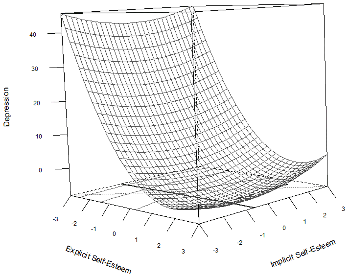
Figure 2
Response surface plot representing the regression equation for the relationship between explicit and implicit self-esteem on depression.
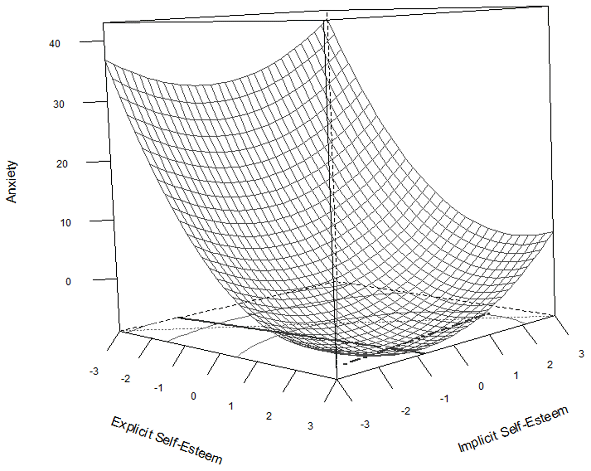
Figure 3
Response surface plot representing the regression equation for the relationship between explicit and implicit self-esteem on anxiety.
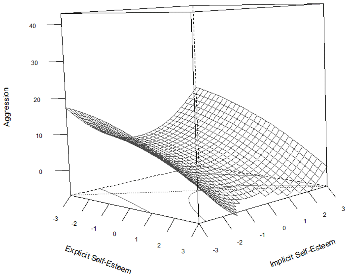
Figure 4
Response surface plot representing the regression equation for the relationship between explicit and implicit self-esteem on aggression.