
Table 1
Descriptive Statistics and Associations between SOCs.
| M ± SD | Skew./Kurt | Decision | Implementation | Maintenance | Habit | |
|---|---|---|---|---|---|---|
| Detection | 3.63 ± 1.97 | 0.03/1.17 | .76* | .47* | .40* | –.33* |
| Decision | 3.72 ± 1.96 | –0.05/–1.19 | .54* | .44* | –.53* | |
| Implementation | 4.16 ± 1.90 | –0.22/–1.01 | .71* | –.33* | ||
| Maintenance | 4.46 ± 1.92 | –0.42/–0.91 | –.21* | |||
| Habit | 4.63 ± 1.94 | –0.29/–1.13 |
[i] Note: M = Mean; SD = Standard Deviation; Skew./Kurt. = Skewness/Kurtosis. Significant relationships (p ≤ .01) denoted with “*”.
Table 2
Descriptive Statistics and Associations between SOC, Motives, and PA Indices.
| M ± SD | Skew./Kurt. | 1 | 2 | 3 | 4 | 5 | 6 | 7 | 8 | 9 | 10 | 11 | 12 | 13 | |
|---|---|---|---|---|---|---|---|---|---|---|---|---|---|---|---|
| 1. SoC | |||||||||||||||
| 2. Intrinsic | 4.57 ± 1.75 | –0.47/–0.54 | .39* | ||||||||||||
| 3. Integrated | 3.61 ± 1.72 | 0.10/–0.77 | .33* | .42* | |||||||||||
| 4. Identified | 5.89 ± 1.24 | –1.29/1.62 | .31* | .26* | .38* | ||||||||||
| 5. Introjected | 3.27 ± 1.75 | 0.30/–0.90 | –.02 | –.01 | .24* | .06 | |||||||||
| 6. External | 3.54 ± 1.78 | 0.15–0.90 | –.01 | .06 | .17* | .07+ | .42* | ||||||||
| 7. Amotivation | 1.67 ± 1.22 | 2.07/4.03 | –.21* | –.10* | .01 | –.28* | .14* | .11* | |||||||
| 8. Aut. motives | 4.69 ± 1.19 | –0.39/0.05 | .45* | .78* | .82* | .66* | .13* | .13* | –.14* | ||||||
| 9. Cont. motives | 3.41 ± 1.49 | 0.12/–0.70 | –.01 | .03 | .24* | .07 | .84* | .85* | .15* | .15* | |||||
| 10. Mild PA | 4.20 ± 3.60 | 2.10/9.58 | .01 | .04 | –.02 | .01 | –.01 | –.04 | –.02 | .02 | .03 | ||||
| 11. Moderate PA | 2.87 ± 2.61 | 1.13/1.81 | .27* | .21* | .16* | .15* | .04 | .00 | –.04 | .23* | .03 | –.02 | |||
| 12. Strenuous PA | 3.41 ± 1.49 | 0.12/–0.70 | .51* | .36* | .32* | .22* | –.01 | .00 | –.09+ | .40* | .00 | .31* | .24* | ||
| 13. MVPA | 25.65 ± 0.71 | 0.71/0.25 | .52* | .38* | .32* | .24* | .02 | .00 | –.09+ | .42* | .01 | .14* | .69* | .87* | |
| 14. PA frequency | 0.78 ± 0.16 | –0.16/–1.36 | .60* | .35* | .37* | .27* | .04 | .02 | –.14* | .44* | .03 | .03 | .34* | .64* | .66* |
[i] Note: M = Mean; SD = Standard Deviation; Skew./Kurt. = Skewness/Kurtosis; Aut. motives = Autonomous motives; Cont. motives = Controlling motives; variables 2–9 ranged from 1–7, mild PA ranged from 0–30, Moderate PA ranged from 0–15, Strenuous PA ranged from 0–10, MVPA ranged from 1–115, and PA frequency ranged from 1–3. Significant relationships (p ≤ .01) denoted with “*”, and significant relationships (p ≤ .05) denoted with a “+”.
Table 3
MANOVAS: Differences in PA Motives across SOCs.
| Det./Dec M ± SD | Implementation M ± SD | Maintenance M ± SD | Habit M ± SD | Pillai’s Trace; ηp2 | |
|---|---|---|---|---|---|
| Intrinsic | 3.42 ± 1.84 | 3.94 ± 1.60 | 4.31 ± 1.62 | 5.38 ± 1.46 | F = (3, 696) = 41.52; p ≤ .001, ηp2 = 0.18 |
| Detection/decision – Maintenance: Games-Howell (ΔM = –0.89), p ≤ .001, g = –0.53 (95% CI = –0.71, –0.34) | |||||
| Detection/decision – Habit: Games-Howell (ΔM = –1.97), p ≤ .001, g = –1.25 (95% CI = –1.40, –1.09) | |||||
| Implementation – Habit: Games-Howell (ΔM = –1.44), p ≤ .001, g = –0.96 (95% CI = –1.12, –0.28) | |||||
| Maintenance – Habit: Games-Howell (ΔM = 1.08), p ≤ .001, g = –0.70 (95% CI = –0.83, –0.56) | |||||
| Integrated | 2.59 ± 1.38 | 3.17 ± 1.42 | 3.47 ± 1.63 | 4.22 ± 1.75 | F = (3, 696) = 5.64; p ≤ .001, ηp2= 0.11 |
| Detection/decision – Implementation: Games-Howell (ΔM = –0.58), p ≤ .05, g = –0.41 (95% CI = –0.62, –0.21) | |||||
| Detection/decision – Maintenance: Games-Howell (ΔM = –0.88), p ≤ .001, g = –0.56 (95% CI = –0.70, –0.40) | |||||
| Detection/decision – Habit: Games-Howell (ΔM = –1.63), p ≤ .001, g = –0.98 (95% CI = –1.15, –0.81) | |||||
| Implementation – Habit: Games-Howell (ΔM = –1.05), p ≤ .001, g = –0.62 (95% CI –0.80 = –0.45) | |||||
| Maintenance – Habit: Games-Howell (ΔM = –0.88), p ≤ .001, g = 0.44 (95% CI = 0.59, 0.30) | |||||
| Identified | 5.04 ± 1.48 | 5.70 ± 1.11 | 5.93 ± 1.23 | 6.22 ± 1.03 | F = (3, 696) = 23.87; p ≤ .001, ηp2= 0.10 |
| Detection/decision – Implementation: Games-Howell (ΔM = –0.66), p ≤ .05, g = –0.50 (95% CI = –0.69, –0.30) | |||||
| Detection/decision – Maintenance: Games-Howell (ΔM = –0.89), p ≤ .001, g = –0.68 (95% CI = –0.82, –0.54) | |||||
| Detection/decision – Habit: Games-Howell (ΔM = –1.18), p ≤ .001, g = –1.01 (95% CI = –1.13, –0.90) | |||||
| Implementation – Habit: Games-Howell (ΔM = –0.52), p ≤ .001, g = –0.50 (95% CI = –0.60, –0.39) | |||||
| Maintenance – Habit: Games-Howell (ΔM = –0.29), p ≤ .001, g = –0.26 (95% CI = –0.36, –0.16) | |||||
| Introjected | 2.94 ± 1.60 | 3.72 ± 1.82 | 3.53 ± 1.68 | 3.05 ± 1.80 | F = (3, 696) = 5.64; p < .001, ηp2= 0.03 |
| Detection/decision – Implementation: Games-Howell (ΔM = –0.78), p ≤ .05, g = 0.42 (95% CI = 0.70, 0.21) | |||||
| Detection/decision – Maintenance: Games-Howell (ΔM = –0.59), p ≤ .05, g = 0.36 (95% CI = 0.53, 0.00) | |||||
| Implementation – Habit: Games-Howell (ΔM = 0.67), p ≤ .05, g =0.37 (95% CI = 0.18, 0.55) | |||||
| Maintenance – Habit: Games-Howell (ΔM = 0.48), p ≤ .01, g = 0.27 (95% CI = 0.12, 0.43) | |||||
| External | 3.38 ± 1.65 | 3.70 ± 1.72 | 3.72 ± 1.70 | 3.40 ± 1.90 | F = (3, 696) = 1.68; p > .05, ηp2= 0.01 |
| Amotivation | 2.16 ± 1.46 | 2.00 ± 1.36 | 1.60 ± 1.05 | 1.46 ± 1.13 | F = (3, 696) = 9.43; p < .001, partial η2 = 0.05 |
| Detection/decision – Maintenance: Games-Howell (ΔM = 0.56), p ≤ .01, g = 0.47 (95% CI = 0.34, 0.60) | |||||
| Detection/decision – Habit: Games-Howell (ΔM = 0.70), p ≤ .001, g = 0.57 (95% CI = 0.45, 0.69) | |||||
| Implementation – Habit: Games-Howell (ΔM = 0.54), p ≤ .01, g = 0.46 (95% CI = 0.33, 0.58) | |||||
[i] Note: Means, standard deviations, Pillai’s Trace, and ηp2 are presented in a single row for each stage of change followed by each individual significant comparison and the corresponding effect size using Hedge’s g.
Table 4
MANOVAS: Differences in PA Indices across SOCs.
| Det./Dec M ± SD | Implementation M ± SD | Maintenance M ± SD | Habit M ± SD | Pillai’s Trace; ηp2 | |
|---|---|---|---|---|---|
| Mild PA | 3.81 ± 3.62 | 4.57 ± 3.97 | 4.36 ± 3.25 | 4.08 ± 3.74 | F(3, 696) = 0.96, p > .05; ηp2 = .004 |
| Moderate PA | 1.61 ± 1.96 | 2.36 ± 2.66 | 2.61 ± 2.51 | 3.68 ± 2.63 | F(3, 696) = 20.14, p ≤ .001; ηp2 = .080 |
| Detection/decision – Maintenance: Games-Howell (ΔM = –1.01), p ≤ .001, g = –0.42 (95% CI = –0.68, –0.17) | |||||
| Detection/decision – Habit: Games-Howell (ΔM = –2.06), p ≤ .001, g = –0.84 (95% CI = –1.08, –0.59) | |||||
| Implementation – Habit: Games-Howell (ΔM = –1.32), p ≤ .001, g = –0.09 (95% CI –0.38, 0.18) | |||||
| Maintenance – Habit: Games-Howell (ΔM = –1.06), p ≤ .001, g = 0.00 (95% CI = –0.22, 0.23) | |||||
| Strenuous PA | 0.47 ± 0.95 | 0.63 ± 1.10 | 1.51 ± 1.74 | 3.39 ± 2.12 | F(3, 696) = 107.27, p ≤ .001; ηp2 = 0.32 |
| Detection/decision – Maintenance: Games-Howell (ΔM = –1.04), p ≤ .001, g = –0.67 (95% CI = –0.84, –0.51) | |||||
| Detection/decision – Habit: Games-Howell (ΔM = –2.92), p ≤ .001, g = –1.55 (95% CI = –1.73, –1.36) | |||||
| Implementation –Maintenance: Games-Howell (ΔM = –0.88), p ≤ .001, g = –0.55 (95% CI = –0.73, –0.37) | |||||
| Implementation – Habit: Games-Howell (ΔM = –2.77), p ≤ .001, g = –1.42 (95% CI = –1.62, –1.22) | |||||
| Maintenance – Habit: Games-Howell (ΔM = –1.89), p ≤ .001, g = –0.96 (95% CI = –1.13, –0.79) | |||||
| PA frequency | 1.35 ± 0.54 | 1.58 ± 0.61 | 1.91 ± 0.69 | 2.65 ± 0.56 | F(3, 696) = 157.38, p ≤ .001; ηp2 = 0.40 |
| Detection/decision – Maintenance: Games-Howell (ΔM = –0.57), p ≤ .001, g = –0.86 (95% CI = –0.93, –0.79) | |||||
| Detection/decision – Habit: Games-Howell (ΔM = –1.30), p ≤ .001, g = –2.34 (95% CI –2.39, –2.28) | |||||
| Implementation –Maintenance: Games-Howell (ΔM = –0.34), p ≤ .001, g = –0.49 (95% CI = –0.57, –0.42) | |||||
| Implementation – Habit: Games-Howell (ΔM = –1.07), p ≤ .001, g = –1.87 (95% CI = –1.93, –1.81) | |||||
| Maintenance – Habit: Games-Howell (ΔM = –0.74), p ≤ .001, g = –1.25 (95% CI –1.31, –1.19) | |||||
[i] Note: Means, standard deviations, Pillai’s Trace, and ηp2 are presented in a single row for each stage of change, followed by each individual significant comparison and the corresponding effect size using Hedge’s.
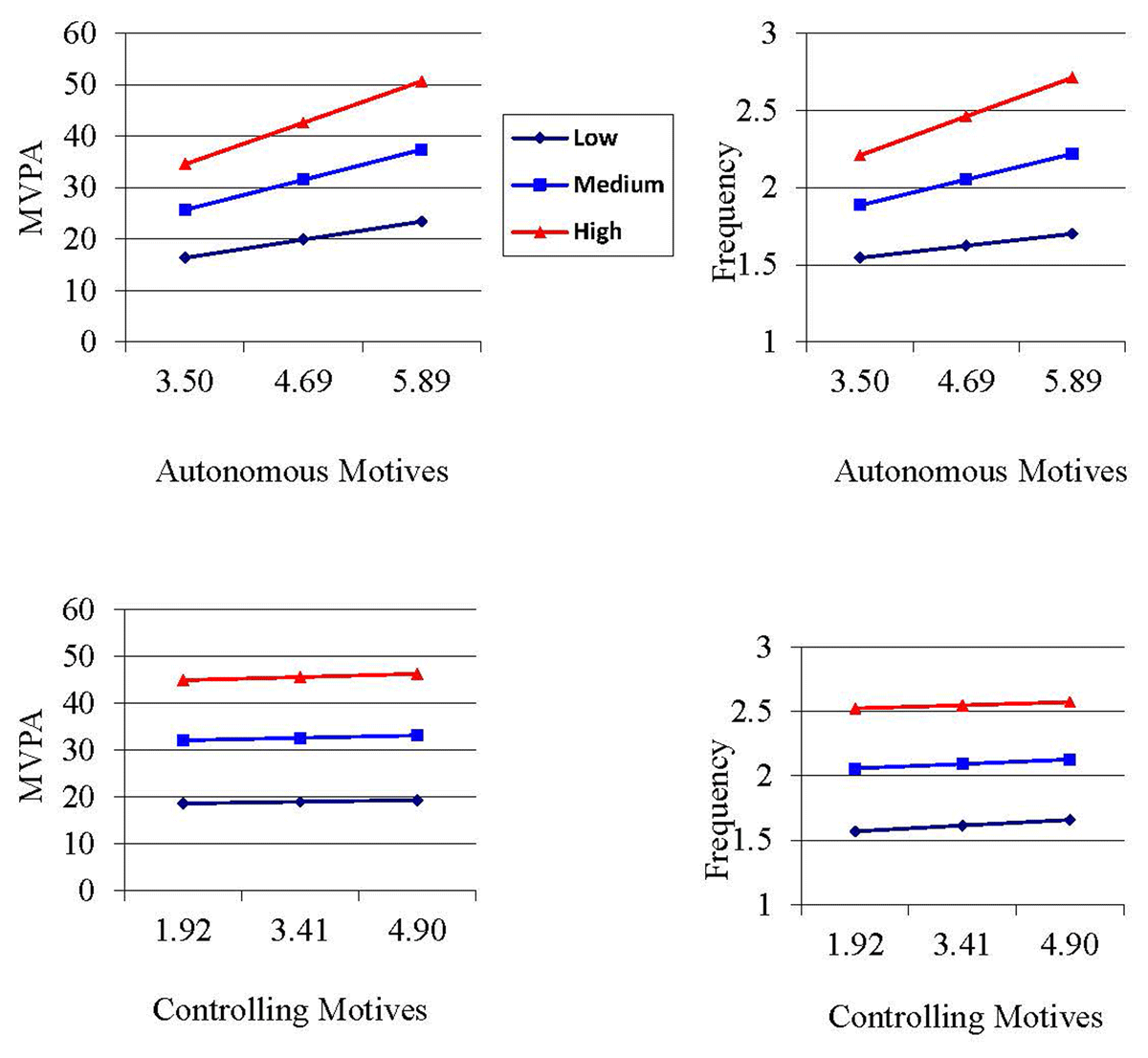
Figure 1
Simples Slops for Regression Analyes with Moderation.