
(1) Overview
Introduction
Diffusion magnetic resonance imaging (dMRI) is a powerful imaging modality that acquires in-depth information about tissue microstructure by tracking the motion of endogenous water molecules under the influence of magnetic field gradients (1, 2). As the water molecules collide with various obstacles in the tissue (e.g., cellular membranes), the dMRI signal attenuates in ways that reflect the underlying tissue structure (3). The attenuation of this signal can be described via mathematical and computational models, with parameters that directly relate to specific features of the tissue (4). Models are often made up of multiple compartments where the dMRI signal is modelled as coming from water in separate microstructural environments (5).
Multi-compartment modelling has played a significant role in recent dMRI research. It has been used extensively in the brain, enabling breakthroughs in understanding the orientation of white matter pathways (6, 7, 8). It has also been used in the body, for example, to understand the composition of tumours in various organs, such as the prostate and kidney (9, 10). The interpretation of the estimated model parameters in relation to tissue composition depends on several factors: the appropriateness of the model for the tissue of interest (11), the sensitivity of the acquisition protocol (12), the specificity of the model’s parameters to the tissue feature of interest (13) and finally, the robustness of the optimisation approach to estimate the parameters from the measured data (14).
Various platforms have released application-specific toolboxes for particular multi-compartment model implementations. Examples include University College London’s (UCL) Camino package for microstructure estimation (15), MRtrix’s work focused on tractography (16) and Dipy’s wide variety of dMRI signal models (17). Additionally, the Dmipy toolbox is a software package that allows the user to implement their own multi-compartment model by combining various approximations of tissue geometries and performing optimisation (18). However, the optimisation methods in these packages are largely based on traditional fitting methods, such as grid search and non-linear optimisation (e.g., Dmipy’s brute2fine function), which are computationally expensive and prone to converging to local minima (19).
To address the limitations of traditional fitting methods, deep learning was proposed as an alternative solution (20). Supervised learning methods have been used widely and typically use large synthetic datasets for training (21, 22, 23). However, this approach can introduce significant biases to parameter estimates (24). Self-supervised approaches mitigate these biases by removing the need for external training data altogether and instead learning patterns from the input data itself over successive iterations (25). Self-supervised learning has shown improved parameter estimation over supervised deep learning for both simple two-compartment models, such as the intravoxel incoherent motion (IVIM) model (26), and more complex models, such as VERDICT (27). The self-supervised approach offers additional advantages—for example, it can naturally handle data with different acquisition protocols or where each voxel has a different effective acquisition protocol, such as after gradient nonuniformity correction.
However, a significant limitation of existing self-supervised dMRI fitting approaches is that, despite often employing the same signal models and machine learning architectures, they are implemented in separate, model-specific codebases. This duplication of effort hinders repeatability, reproducibility and the development of new methods. To address this, we present microTorch, an open-source software package that provides a modular framework for self-supervised model fitting across a host of dMRI signal models and neural network architectures. By unifying within a common framework, microTorch makes the speed and performance advantages of self-supervised model fitting accessible to the wider quantitative MRI community. In its current form, microTorch supports inference on user data for most established dMRI models or combinations of their constituent compartments. The package is designed to be easily extensible, and we aim to continually extend its coverage and capabilities through future development and contributions from the community.
Implementation and architecture
Software architecture
microTorch is implemented as a layered, modular software structure designed to maximise maintainability, extensibility and ease of use (Figure 1). At the top level, microTorch is divided into several directories with distinct purposes. The examples directory contains Jupyter notebooks that demonstrate package functionality, whilst simulation_data stores example synthetic datasets used for testing and validation. The scripts directory stores standalone workflow scripts, the tests directory contains the automated test suite used to verify expected behaviour, and the docs directory contains the project documentation. Separating these components avoids mixing the main package code with examples, data, testing infrastructure, and explanatory material.
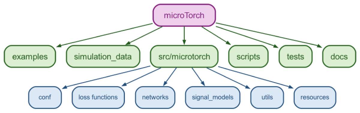
Figure 1
microTorch package structure. Top level (green) includes the package source code (src/microtorch) alongside example notebooks, simulated data, scripts, tests and documentation. The source code (blue) contains configuration files, loss functions, neural networks, signal model classes, helper functions (in utils) and package data (in resources).
The main implementation is contained within src/microtorch, which forms the core Python package installed when users run pip install microTorch-MRI. Using an src layout ensures that imports resolve to the installed package and that local development mirrors how users will interact with the installed package. It also ensures that only the core package is distributed during installation, whilst examples, documentation, tests, scripts, and demonstration data remain part of the source repository.
Within src/microtorch, the code is arranged by functionality. The conf directory contains configuration files, enabling acquisition, model, training and optimisation settings to be changed seamlessly. The loss_functions and networks directories contain reusable machine learning components, making it straightforward to interchange architectures and loss functions or add new ones. The signal_models directory contains dMRI signal models and is organised to enable the addition of new models with minimal modification to the surrounding code. The utils directory provides shared helper functions, whilst the resources directory stores package data, such as example acquisition protocols, which must be distributed with the software.
This design enables development in multiple directions without affecting unrelated components. For example, new signal models can be added to signal_models, new neural network architectures to networks, or additional acquisition protocols to resources, without requiring major changes elsewhere in the codebase.
Acquisition protocol handling
dMRI scans comprise a series of volumes acquired with different diffusion weightings, where the diffusion weighting of each volume is determined by acquisition parameters that control the sensitivity to molecular diffusion and hence information on tissue properties (28). Such acquisition parameters include the gradient directions (or b-vectors) and b-values, with the b-value further decomposed into the gradient strength, G, the duration of each gradient pulse, δ, and the time between the onset of each pulse, Δ (29).
microTorch stores acquisition parameters in the AcquisitionScheme module. The AcquisitionScheme module takes input dMRI acquisition parameters and processes them into a common fixed structure that can be passed to corresponding model functions to be used for signal generation. There are two ways of instantiating a microTorch AcquisitionScheme object:
– Using MRtrix-style (16) ‘grad’ text files, which include one row per diffusion-weighted volume, with gradient directions in the first three columns and b-values in the fourth. We extend this format in microTorch to optionally include Δ, δ, and echo time (TE) in additional columns for models that require these acquisition parameters.
– Using FMRIB Software Library (FSL)-style (30) separate b-value and b-vector text files and, optionally, Δ, δ, and TE text files.
A series of validation checks is performed on the acquisition scheme parameters to ensure the input dimensions are correct and that values are non-negative. For example, in the case of the ‘grad’ file input, acquisition parameters must adhere to the pre-defined column ordering (i.e., gradient directions, b-values Δ, δ,TE).
Signal model framework
To estimate specific properties of the tissue microstructure, multi-compartment models represent the tissue as a linear combination of single-compartment models, each representing the diffusion signal originating from a certain tissue type. The recovery of microstructural information is achieved by estimating the model parameters that minimise an objective function (typically mean-squared error (MSE)) describing how well the modelled dMRI signal aligns with the measured signal over all acquisition parameters. For these model parameters to accurately describe the tissue in question, it is essential that the composition of the multi-compartment model (in terms of the chosen tissue geometries) is appropriate for the actual tissue composition.
In microTorch, the separate building blocks that make up the multi-compartment model are represented using Python classes. These classes encode the signal equation of a single biophysical compartment model. By combining these compartment signal models in various combinations, one can construct almost any multi-compartment model in the literature.
The compartment signal model classes are initialised with the parameter names, number of parameters, and their biophysically reasonable estimation ranges. Predicted signal data for a compartment model is generated by calling an instance of the compartment class, which evaluates the corresponding signal equation. This requires values for the model parameters and acquisition parameters, provided as a PyTorch tensor and an AcquisitionScheme object, respectively. The acquisition parameters are extracted from the AcquisitionScheme object and, together with the model parameters, passed to the compartment equation to produce signal values.
The signal attenuation of a compartment can be represented in two ways: a directional representation—considering all gradient directions and fitting a directional model—or a spherical mean representation, where measurements are averaged over all gradient directions before fitting a spherical mean model. This property is stored in each compartment signal model class, as multi-compartment models cannot combine spherical mean and directional compartments (although some compartments, such as ‘Ball’, support both).
The microTorch ModelMaker module combines these separate compartment signal model classes into a multi-compartment model class. The ModelMaker module can either take as input the name of an established model from literature (e.g., VERDICT) and retrieve its constituent compartment classes (Ball, Sphere, Astrosticks), or be given any combination of compartments in Pascal case (e.g., BallSphere) and return the overall multi-compartment model signal. ModelMaker maps the model name to the appropriate compartment classes, validates the consistency of the spherical mean property across the compartment classes, retrieves parameter properties for each compartment, and then creates a multi-compartment model class representing the full model. The multi-compartment model class initialises the parameter names, number of parameters, and estimation ranges by combining those from each constituent compartment class. It also adds one volume fraction parameter per compartment. Parameter ordering in tensors defining names, ranges and values follows the order in which compartments are passed to ModelMaker. For example, BallSphere places Ball parameters first, followed by Sphere parameters, and then the Ball and Sphere volume fractions, respectively. Calling an instance of the multi-compartment model class with an AcqusitionScheme object and model parameters (including volume fractions) as input computes the overall model-predicted signal by weighting each compartment’s signal contribution by its volume fraction.
Microstructure models are typically either signal representation-based, which model the diffusion MRI signal using mathematical expansions, or biophysical, based on tissue geometrical properties consistent with histology. In microTorch, we include examples of both; these can be found within src/microtorch/signal_models.
Gaussian models are used to represent free or hindered diffusion inside tissues that are not explicitly restricting the movement of diffusing particles. In microTorch, we include the Ball (7), Zeppelin (31) and Tensor (6) Gaussian models in the gaussian_models.py file. Restricted diffusion models describe particles that, during the pulse separation time Δ, diffuse through tissue until they encounter enclosing boundaries that they cannot cross. We include the Cylinder (31), Stick (7) and Astrosticks (9) in the cylinder_models.py file, and the Sphere (32) and Dot (31) restricted models in the sphere_models.py file. In the future, we will also include the standard model for white matter (33) and further distributed models. Each of these models is implemented as a Python class with biophysically reasonable parameter constraints enforced.
These compartments can be combined to form widely used multi-compartment models. For example, both the VERDICT model for prostate and the SANDI (34) model for grey matter use the Ball, Sphere and Astrosticks compartments, whilst the IVIM model can be created using two Ball compartments with parameter ranges adjustable via configuration files. Alternatively, new compartment combinations can be created on the fly by combining compartments as the user wishes to explore what best describes their dataset. This can be done by simply listing the separate compartment names in Pascal case (e.g., BallZeppelin), allowing for novel combinations to be trialled for different organs and diseases.
Users can specify custom parameter ranges that override the default biophysically reasonable estimation ranges defined in each compartment class. Parameters can also be fixed to user-defined values rather than estimated, in which case the signal module will use the fixed value. Parameter ranges and fixed values can be configured via a YAML file named after the model and placed in src/microtorch/conf/model. If a specified model does not have an associated YAML file, it defaults to the parameter ranges defined for each of its constituent compartments. Example YAML files for common models are provided. The estimation is constrained to the defined ranges using either the PyTorch ‘clamp’ or ‘sigmoid’ functions, as selected by the user. Volume fraction parameters are additionally constrained to sum to 1, either by a softmax function or by restricting them to between 0 and 1 (using clamp or sigmoid), followed by normalisation.
Optimisation framework
To estimate the unfixed (‘free’) model parameters, an optimisation procedure is performed to minimise a loss function between the model-predicted signal and the measured data. The resulting model parameter values are the optimal estimates.
Self-supervised methods minimise the difference between the noisy MR signals (network inputs) and noise-free predicted signal reconstructed from the model parameters (network outputs) (25). The training loss is between the predicted signal, Ŝ, and the input signal, S (26). Training and inference are performed in tandem on the dataset of interest, removing the requirement for separate training and testing datasets.
microTorch implements a default fully-connected feedforward network with three hidden layers, each with 256 neurons. Network definitions are stored in microTorch/networks, and users can add their own custom architectures to this directory. Ongoing work is focused on extending the framework to include variational autoencoders and convolutional neural networks. The output layer has one neuron per model parameter to be estimated. The output layer signal model equation generates the predicted signal—see Figure 2. Crucially, this requires coding the signal model in PyTorch in a fully differentiable form. Each compartment’s signal equation is defined as a PyTorch tensor function within its class. This allows multidimensional tensors of batched parameter values to be passed to the classes, yielding batched tensors of predicted signals, Ŝ. We use the ADAM optimiser and optimise the network by backpropagating the reconstruction loss between the input signal (S) and predicted signal (Ŝ). For the final parameter estimation, we use the network at the epoch with minimum reconstruction loss (26).
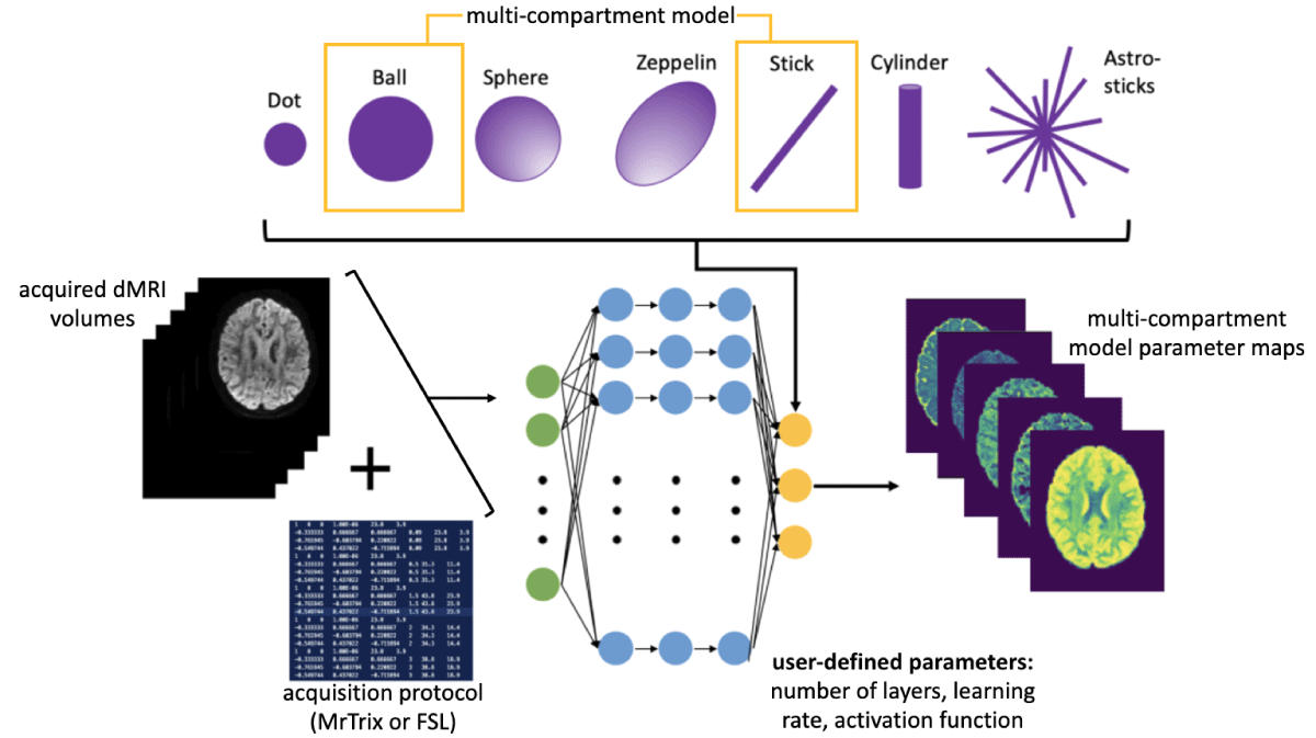
Figure 2
Overview of the microTorch fitting procedure. Acquired dMRI data are fed into the network at the input layer (green nodes) and passed through multiple hidden layers (blue nodes). The final layer implements the desired compartment model signal equation in PyTorch, taking the model parameters and associated acquisition protocol parameters as input to generate a synthetic signal. The loss between this synthetic signal and the measured signal is then minimised, ensuring that the network (yellow output layer) learns the underlying model parameters.
The neural network is created for each multi-compartment model via the microTorch Net module, which flexibly embeds the signal model within the forward pass. This allows any compartment model, defined via its corresponding class, to be used for predicting the dMRI signal and estimating microstructure model parameters. The network architecture and training settings—including layers, activation functions, learning rate, constraint methods, dropout, loss function, batch size, maximum epochs and patience for early stopping—are configurable via YAML files in src/microtorch/conf/training, with options to override these via the command-line interface.
Configuration and experiment management
The microTorch package allows users to tune hyperparameters before fitting the final model. The hyperparameters available for tuning are the number of layers, the number of hidden neurons, patience, dropout rate, learning rate and the activation function. Users can specify the values to explore for each hyperparameter by setting the desired ranges in the appropriate YAML configuration file located in the src/microtorch/conf/tuning folder.
Tuning is performed using the Optuna framework (35), which employs a Bayesian optimisation strategy for the efficient exploration of the search space via the Tree-structured Parzen Estimator (TPE). The number of trials run by Optuna defaults to 40, but users can specify a custom number. The objective metric being minimised is the training loss. A Median Pruner is also implemented to interrupt trials that show insufficient promise relative to previously completed trials. The Median Pruner does not intervene during the first five trials (controlled by the n_startup_trials parameter) and waits until at least 100 epochs have elapsed within a trial before pruning (controlled by the n_warmup_steps parameter).
Extending microTorch
We anticipate that contributions will usually involve the addition of new signal models, tissue compartments, or neural network architectures. Contributors are encouraged to fork the repository, create a feature branch, implement their changes and submit a pull request. Detailed contribution guidelines, together with examples, are provided in docs/developer. To ensure quality control, we included a GitHub Actions workflow in .github/workflows that automatically runs code linting with Ruff and the full test suite with coverage across Python 3.9, 3.10 and 3.11 for every push and pull request.
Validation and testing
The package contains a full testing suite within microtorch/tests. The tests are run via pytest, and include simple mechanisms for testing utils functions, signal models, network and training functions, and acquisition scheme handling. Test coverage is assessed using pytest-cov. The current coverage of in-scope modules is 94%, whilst excluded modules and the rationale for their exclusion are documented in docs/developer/testing.md. For the larger building blocks of the model fitting, we include an integration test in tests/integration, which simulates ground truth data, fits the models and asserts that the fitted parameters recover the ground truth with a correlation above 0.85. We encourage users who wish to add a signal model to the package to include appropriate unit tests to check its functionality.
Additionally, we provide methods for the user to trial the package with simulated data prior to using it on their own data. The create_test_images.py file can be run to simulate test data for a given model, and the create_all_test_images.py script will generate test data for all multi-compartment models currently defined in the package. The user can then run the fitting procedure on this test data as outlined in the documentation. We also include Jupyter notebook examples (microtorch/examples) that demonstrate how best to use the package for simple fitting tasks with a test image and example acquisition scheme.
Documentation, including how to run on the provided simulated data and on your own data, is provided in the README.md. Detailed docstrings are provided with each function explaining their use.
(2) Availability
Operating system
MacOS: 10.15+
Linux: 18.04+
Windows: Windows 10
Programming language
Python 3.8+ (PyTorch 2.x)
Additional system requirements
– Hardware: 64-bit processor (2+ cores recommended)
– Memory: Minimum 4 GB RAM (8–16 GB recommended for large diffusion MRI datasets)
– Disc Space: <1MB for installation of the package itself, up to 2GB for dependencies (PyTorch) and additional space required for input datasets
Dependencies
Core dependencies: torch, numpy, nibabel, tqdm, SciPy, matplotlib, torchmetrics, hydra-core, Jupyter, Optuna
Development dependencies: PyTest, PyTest-Cov, Ruff
List of contributors
Snigdha Sen, Paddy J Slator, Gerrit C Arends, Marta Masramon, Rajib Ahmed, Christopher S Parker, Marco Palombo, Alvaro Planchuelo Gomez and Nicola Casali.
Software location
Code repository (e.g., SourceForge, GitHub etc.)
Name: GitHub
Identifier: snigdha-sen/microtorch
Licence: MIT
Date published: 30/04/2026
Language
Python, Shell
(3) Reuse Potential
Within the field, this package can be used for fast and robust parameter estimation of multiple microstructural diffusion MRI models to various datasets. We envisage microTorch eventually encompassing most modelling requirements in the dMRI field, with immediate plans in place for the inclusion of the NODDI (36) model. These developments can be added to the repository via GitHub’s pull request feature and will be reviewed by a member of the team. The development team also has plans in further versions to include different fitting strategies for comparison—for example, with different deep learning approaches (37). Contributors can contact the lead author via email, which is included in the README.md. Although microTorch was developed for dMRI model fitting, many other quantitative MRI (qMRI) applications, including T1 and T2 mapping, arterial spin labelling (ASL), and MR elastography, follow the same model fitting paradigm and could therefore be readily supported with the addition of appropriate signal model implementations. Moreover, the self-supervised fitting method can be a source of inspiration for other types of model fitting.
Acknowledgements
The authors would like to acknowledge the support of the CUBRIC and Hawkes Medical Imaging Hackathons for providing the environment to collaborate on this project, and members of project teams during these Hackathons who helped the software package take shape.
Author Contributions
Snigdha Sen: Conceptualisation, technical development, paper writing.
Rajib Ahmed: Technical development.
Gerrit C. Arends: Technical development.
Alvaro Planchuelo Gomez: Technical development.
Xiaoxiang Chen: Technical development.
Marta Masramon: Technical development.
Nicola Casali: Technical development.
Marco Palombo: Conceptualisation, technical development, paper review.
Christopher S. Parker: Technical development.
Chantal M. W. Tax: Conceptualisation.
Eleftheria Panagiotaki: Conceptualisation, paper review.
Paddy J. Slator: Conceptualisation, technical development, paper review.