Simulation Software for the Virtual Design and Analysis of Magnetic Sensor Systems

Introduction

Simulations play a crucial role in the development of magnetic sensor technology. A notable application highlighted in this article is the design of magnetic gear and gear rack encoders. These sensors are used to precisely determine the position and velocity of a soft magnetic tooth structure by capturing the modulation of the magnetic field as the tooth structure moves. Giant Magnetoresistance (GMR) elements are commonly used in these systems. These elements change their electrical resistance in response to an external magnetic field. Typically, eight GMR elements are combined to form a single sensor, creating two separate measurement bridges that result in two distinct sensor output signals. Further information and examples of this sensor technology can be found on the Sensitec GmbH website.¹

There is a strong relationship between the geometric properties of the measured object and the arrangement of the GMR elements within the sensor. The dimensions and positioning of these elements must be precisely aligned with the tooth structure to ensure stable sensor signals and maximize system accuracy. System performance is assessed using an error curve to evaluate the overall accuracy.

In reality, this adaptation is only possible to a limited extent for physical objects, and it is very time consuming and costly. In order to be able to test different configurations, prototypes of the sensor technology would have to be manufactured in different versions for each system. Due to production-related fluctuations, some system parameters can only be controlled to a limited extent. The sensor behaviour can deviate significantly due to these inaccuracies. Therefore, real-world system evaluation is only feasible statistically with large quantities. Simulative methods address this challenge by eliminating the need for physical prototypes. System parameters can be precisely determined and effortlessly adjusted to investigate different system configurations under various conditions. The only limitation is the available computing capacity.

Existing simulation software packages already used in production are not suitable for the specific application. The problems are demonstrated using two examples.

Ansys Maxwell is a software for the investigation of electromagnetic fields with the use of the finite element method (FEM) [1]. The software does not allow a holistic system analysis from the magnetic field to the error curve. In addition, the operation of this simulation software is complex and time-consuming, even for simple problems. High demands on the computer hardware further limit the range of application.

Comsol Multiphysics is a multiphysics software that also enables the calculation of physical models with the help of the FEM [2]. The main problem is the complexity of modelling the sensor behaviour. The calculation of the error curve is not possible within the software environment. The presented simulation software are also characterised by high licence fees.

The software presented below for the 3D simulation of magnetic fields and sensors addresses the limitations and weaknesses that exist in existing applications. It combines maximum design freedom and simple operability with the possibility of a holistic system analysis. Important metrics are already implemented and preconfigured. All other system variables are freely accessible and can be used for analysis and evaluation. In addition, the software is open source and published without fees.

Description

The software allows the simulation of three dimensional magnetostatic problems of macroscopic systems with multiple elements of hard or soft magnetic objects and sensors. Hard magnetic materials remain permanently magnetic after magnetisation, while soft magnetic materials slightly change or lose their magnetisation.

The hard magnetic objects included are cuboid, rod and diametral magnets. Soft magnetic objects include gears, gear racks and shafts. Magnetic sensors are implemented as GMR encoders and Hall effect sensors. In addition, the possibility to generate a homogeneous magnetic field that interacts with the physical objects is implemented.

Hard and soft magnetic objects are defined by their shape, position, and orientation in 3D space. Additionally, they are characterized by their relative permeability, and in the case of hard magnetic objects, their magnetization amount and direction. Soft magnetic objects can exhibit time-dependent behaviour. For example, gears can rotate and gear racks can translate. The simulation of dynamic processes is carried out as a consecutive simulation of discrete, time-independent systems. Modelling of the sensor systems is based on physical relationships and empirical characteristics. The models take the magnetic field quantities as inputs and generate the sensor output signals.

A sample setup consisiting of a cuboid magnet, a GMR encoder and a gear is given in Figure 1. A rotating gear with high permeability modulates the magnetic field emanating from the cuboid magnet. The sensor and magnet are positioned just above the tip diameter. Several GMR elements in the sensor detect the modulations and generate output signals in time, indicating the gear angle and speed.

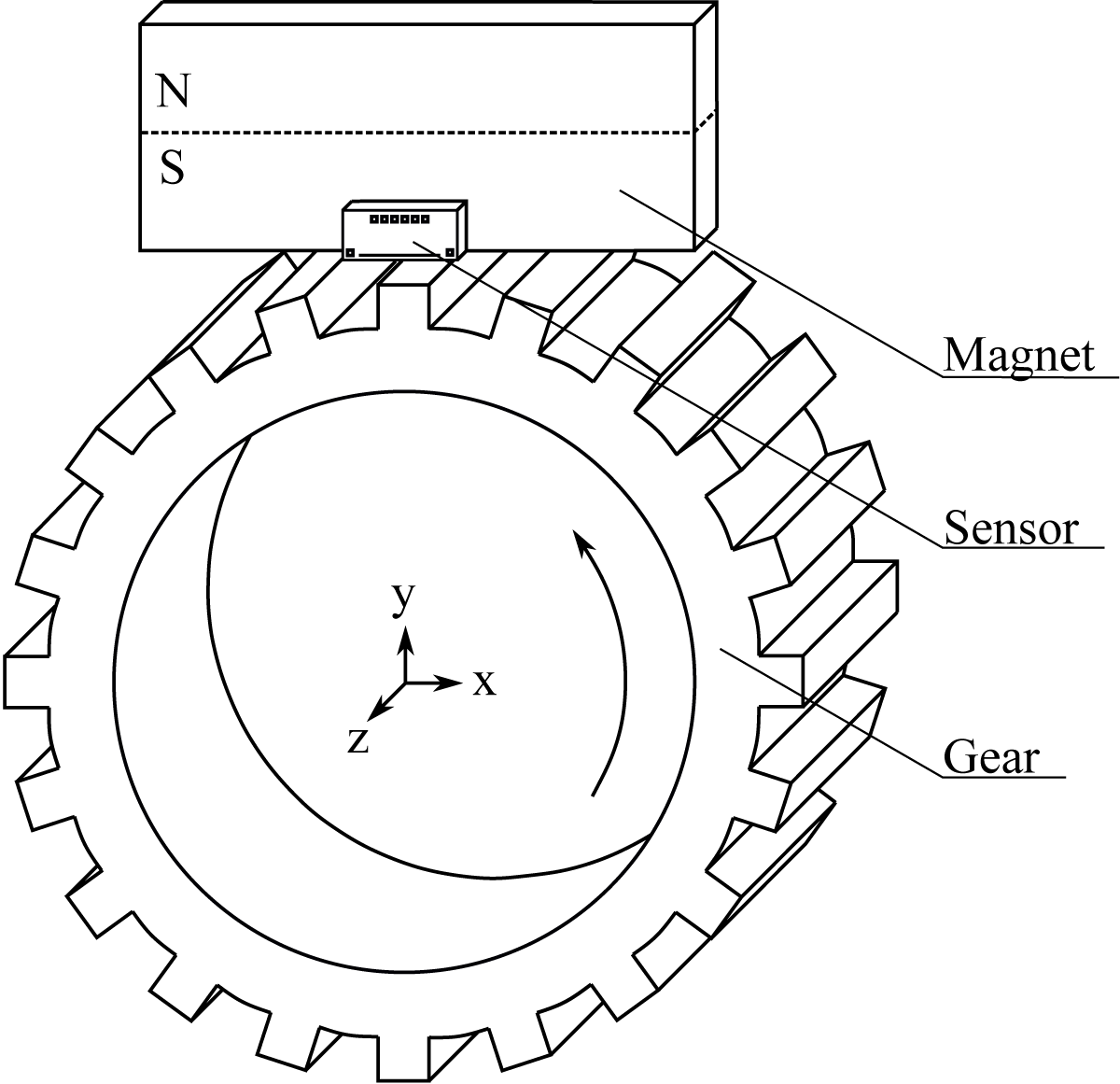
Figure 1

Software Operation

The focus of the development has been on an intuitive user interface to lower the barrier to entry. An image of the Graphical user interface (GUI) is shown in Figure 2.

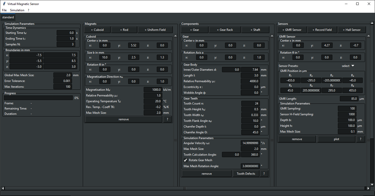
Figure 2

Several common data formats are supported. Metadata can be saved and loaded into the program in the formats HDF5 (Hierarchical data format) [3], INI and in the form of dictionaries in Python scripts (PY). The measurement data is stored together with the metadata exclusively in the HDF5 format. HDF5 is a widely used standard for scientific data management and is supported by many common analysis programs (such as MATLAB for example).

The structure of the GUI is based on the guidelines of the Common user access (CUA) specifications [4]. Guidelines such as keyboard shortcuts or the menu bar are defined by the standard. Users are familiar with the standards from other applications, which lowers the barrier to entry.

All application functions are accessible from a menu bar at the top of the screen. This includes creating new projects, saving and loading files, an options menu, starting the simulation and accessing help options such as the software documentation.

All simulation elements can be easily configured using various parameters. The names of the system parameters are also based on common standards (e.g. DIN ISO 21771 [5]). A parameter is described by a formula symbol and a short description or name. The units are also given. For example, the angular velocity of a gear is given as Angular Velocity, the formula symbol ω and the unit Deg/s. Technical drawings, which can be called up in the programme, further facilitate the assignment of parameters.

The parameters are grouped hierarchically according to their association. For example, the parameters number of teeth n, tooth height h_p, tooth width s_p, tooth flank angle α_p, tooth chamfer depth t and tooth chamfer angle Θ form the group Gear teeth, which belongs to the simulation object Gears. The simulation elements themselves are divided into the main groups hard magnetic elements, components (soft magnetic elements) and sensors.

Dynamic lists allow simulation elements to be added and removed from each of the three main groups. This allows an individual configuration to be created from a selectable number of simulation elements.

Operation is further facilitated by a progress bar that displays the progress of the simulation, including elapsed time and estimated remaining time.

Implementation and architecture

The software was implemented using Python. FEM tools are provided by the multiphysics software library NGSolve [6]. As shown in the following section, the use of the NGSolve functionalities is separated from the rest of the code by an interface.

Figure 3 shows a simplified Unified modeling language (UML) class diagram that illustrates the package structure and the most important relationships between the different classes. All multiplicities are one, unless otherwise stated. The illustration of the relationships between the classes of the GUI is omitted entirely.

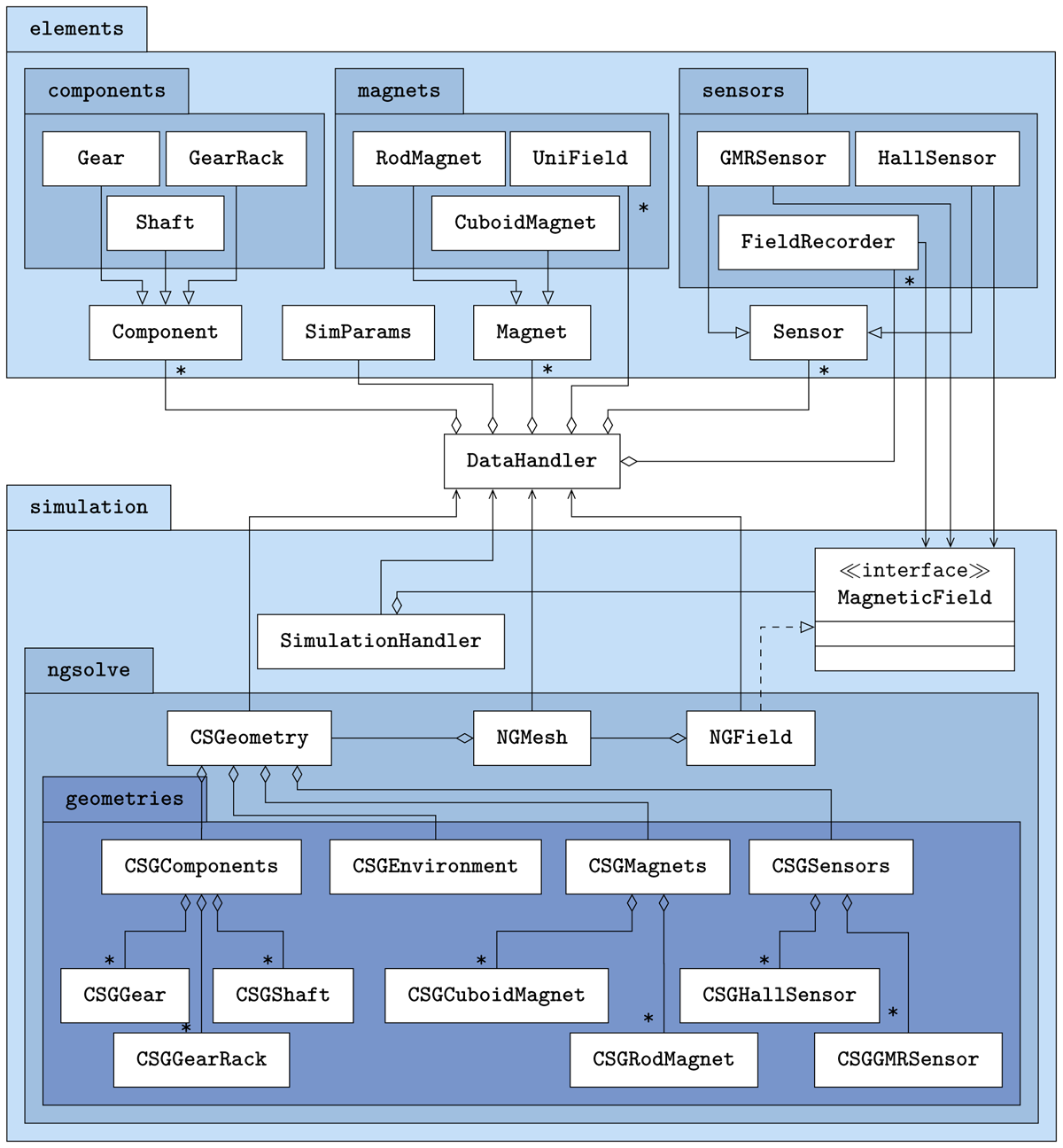
Figure 3

The classes are distributed in two parent packages. The elements package contains the simulation objects and parameters, while the simulation package contains the classes that compute the magnetic field and run the simulation. The link between the two packages is provided by the DataHandler class. It manages all the objects of the classes in the elements package and communicates the information to the classes in the simulation package.

Each physical object that can be modelled in the simulation is represented by its own class in the elements package. There are also classes for generating homogeneous magnetic fields and for recording the magnetic field quantities. All classes are sorted into different packages according to their category. The components package contains the soft magnetic objects, the magnets package contains the hard magnetic objects and the homogeneous magnetic field, and the sensors package contains the sensors and the class for recording the magnetic field quantities. Each package has a superclass from which the classes in the packages inherit attributes and methods. Exceptions are the classes Unifield and FieldRecorder. They do not inherit from the superclass because they do not have physical bodies like regular magnets or sensors.

At the same level as the superclasses there is another class called SimParams. It manages the simulation parameters such as the time sampling rate or the size of the simulation space. The DataHandler class holds any number of superclass objects, but only one SimParams object.

The simulation package contains the classes used to compute the magnetic field. The simulation is performed by methods in the SimulationHandler class. For this purpose, an object of the MagneticField class is created in it. The SimulationHandler class is the only class in the simulation package that communicates with the DataHandler class. The measurement results from the simulation run are passed to the DataHandler class. All other classes in the simulation package only receive data from the DataHandler class.

All classes that refer to the NGSolve library are in the ngsolve package. In order to calculate a magnetic field, two requirements must be met: The geometry of the physical objects must be modelled using Constructive Solid Geometry (CSG) methods and transformed into a mesh suitable for FEM calculations. These tasks are performed by the classes CSGGeometry and NGMesh. For this purpose, objects of the classes CSGComponents, CSGEnvironment, CSGMagnets and CSGSensors are initialised in the class CSGeometry. They manage the physical modelling of the respective simulation objects, which in turn are created in corresponding classes in the geometries package. Each object of the classes CSGGear, CSGShaft, CSGGearRack, CSGCuboidMagnet, CSGRodMagnet, CSGGMRSensor and CSGHallSensor accesses an object of the corresponding class to retrieve geometry information. The connections have been omitted from the diagram for clarity.

The generated mesh is used in the NGField class to calculate the magnetic field. This class implements methods defined abstractly in the MagnetField class. It provides the interface to the classes that refer to the NGSolve library. This completely decouples NGSolve from the rest of the software and allows the simple implementation of other FEM libraries if required. The methods that need to be implemented are defined in the MagnetField class. The GMRSensor, FieldRecorder and HallSensor classes access the MagneticField interface in the simulation package to update their measurement data during the simulation run.

The calculation of the magnetic field quantities is done by solving the POISSON equation of magnetostatics [7]

in its weak form iteratively on a mesh generated by the 2D/3D-mesh generator NETGEN [8]. The vector potential $\overrightarrow{A}$ is linked to the physical fields $\overrightarrow{B}$ and $\overrightarrow{H}$ by the relations

The intermediate step via the vector potential has been taken to decouple the coupled MAXWELL equations and to transform them into a second order differential equation (eq. 1). The magnetisation $\overrightarrow{M}(\overrightarrow{x})$ and the permeability $\mu (\overrightarrow{x})$ are position-dependent functions of the material properties. These properties are given in the appropriate classes.

Quality control

The software is tested using unit, integration, end-to-end and manual tests.

The test suite consists mainly of unit tests and some integration tests to check that the simulation elements are implemented correctly and that data can be saved/loaded to/from disk. In particular, the conversion of SI units to units used in the GUI is a source of incorrect values and is tested for each object. Other methods are checked against known analytical solutions. Backward compatibility checks are included to ensure functionality with legacy measurement and configuration data in current releases.

An end-to-end test ensures that the GUI opens, the simulation runs and the metadata and measurement data are stored correctly on disk.

GUI testing is not yet implemented and will be added in the future. The GUI functionality is tested by manual testing.

The users can run the testsuite themselves by running pytest in the source directory or simply by running the default loaded configuration supplied with the software. By running this configuration, the user can determine whether the software runs without problems and whether the measurement results are saved. The configuration loaded at startup can be changed in the settings menu if desired.

The simulation results are verified using known closed-form analytical solutions. The investigations were carried out on cuboid magnets [910], rod magnets or diametral magnets [11] and soft magnetic cylindrical bodies in arbitrary external fields [1213]. As an example, the comparison between the analytical solution and the simulation solution of a system consisting of a soft magnetic cylinder in a homogeneous external field is shown in Figure 4. The soft magnetic cylinder with a relative permeability of μ_r = 4000, a radius of R = 40mm and a length of l = 30mm is placed in a homogeneous magnetic field with a magnetic flux density of B₀ = 100mT in the y-direction. The Figure 4 compares the magnitudes of the magnetic flux density along the x-axis for different positions along y. All three sections pass through the cylinder. The study shows the consistency of the FE calculations with the analytical solution in the case of soft magnetic objects in external magnetic fields. The remaining deviations are due to numerical inaccuracies. The comparisons between the FE calculations and the analytical solutions in the case of permanent magnets show a similar picture.

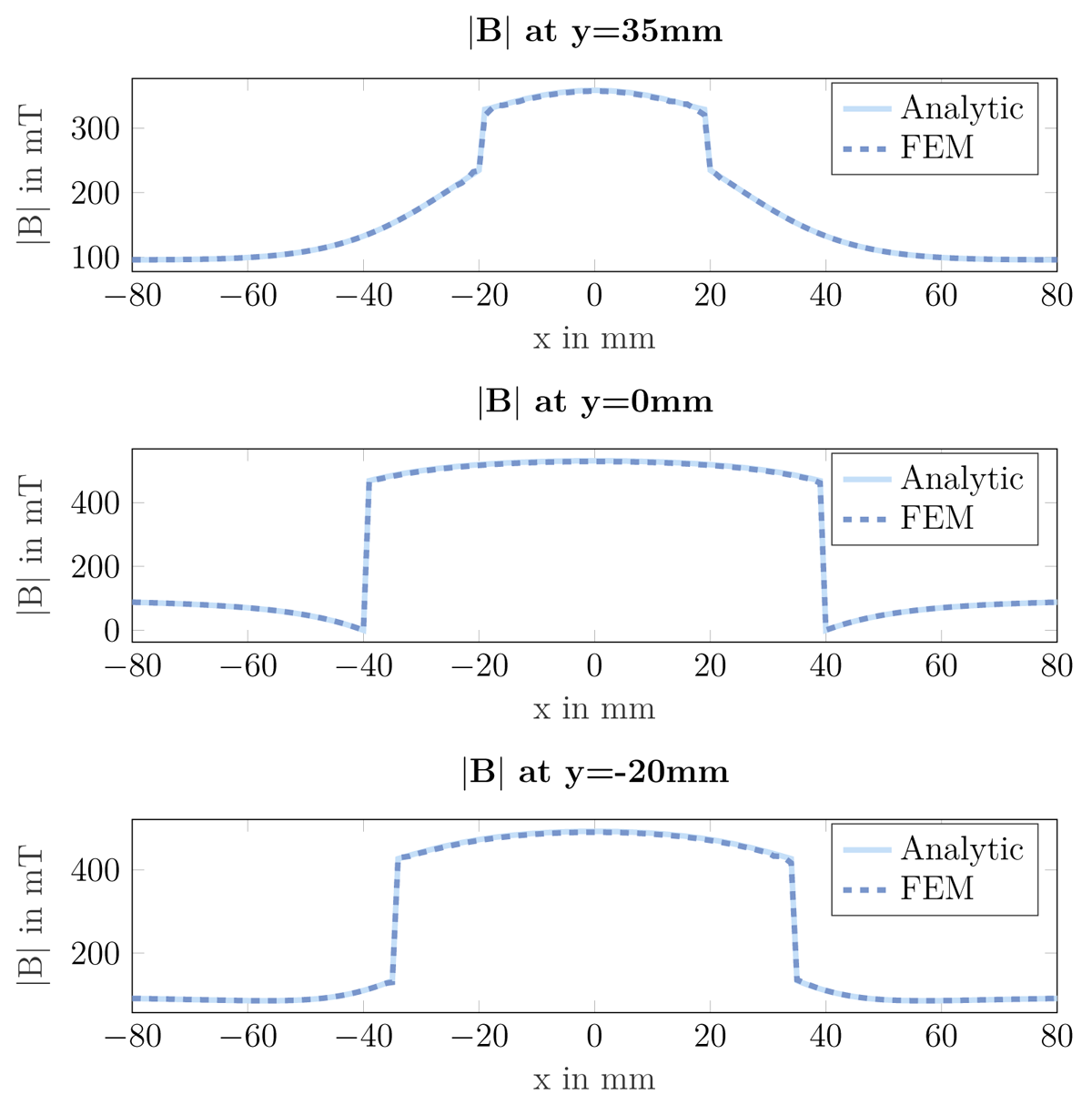
Figure 4

Operating system

Available on any platform that provides a Python compiler.

Tested on Microsoft Windows 10, Windows 11, Ubuntu 24.04 and macOS 13.6.

Programming language

Python 3.10

Dependencies

NGSolve 6.2.2102Netgen 6.2.2102NumPy 1.18.1matplotlib 3.1.3h5py 2.10.0Pillow 7.0.0psutil 5.6.7

Software location:

Archive

• Name: Release 1.0.3

• Persistent identifier: https://doi.org/10.5281/zenodo.8414074

• Licence: LGPL 2.1

• Publisher: Institute of Measurement and Sensor Technology, RPTU University Kaiserslautern-Landau

• Version published: 1.0.3

• Date published: 14/08/25

Code repository

• Name: Virtual Magnetic Sensor

• Persistent identifier: https://github.com/mts-public/virtual_magnetic_sensor

• Licence: LGPL 2.1

• Date published: 04/10/23

Language

English