
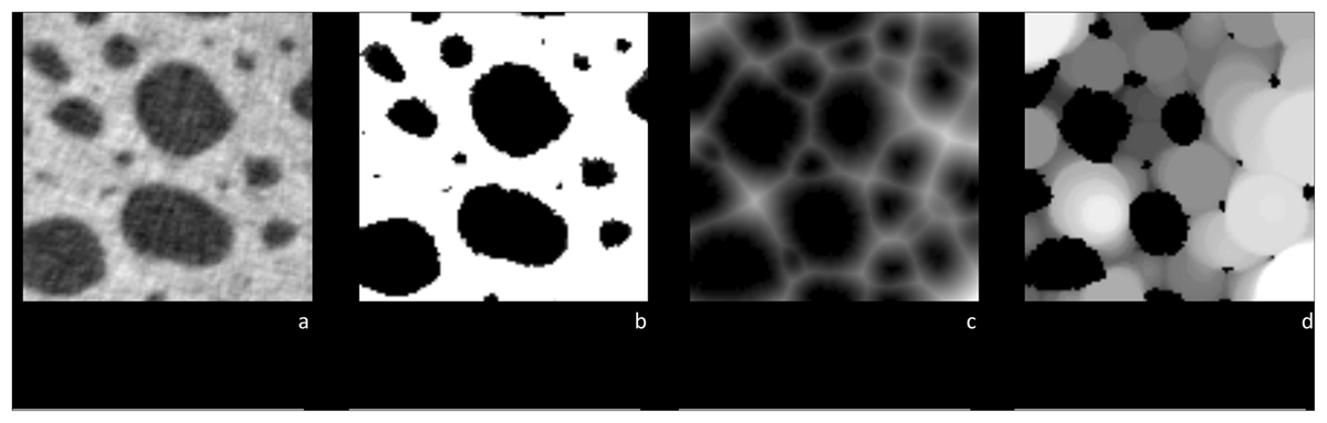
Figure 1
Example of a trabecular bone with a scale bar of 2mm and the respective measurements. a) Trabecular bone b) Binary mask c) Distance map d) Local thickness map.
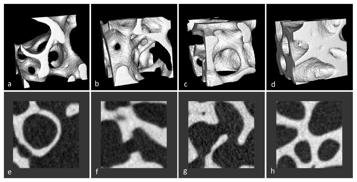
Figure 2
Examples of bone images with different forms and trabecular thickness. 3D rendering (upper panel) and 2D axial slice view (lower panel), respectively.
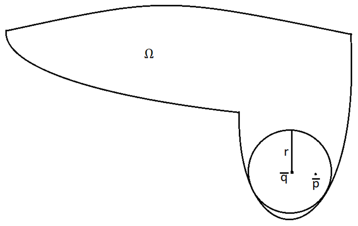
Figure 3
A surface of the object Ω. Measurement of volume-based thickness at the point inside a surface of the object Ω.
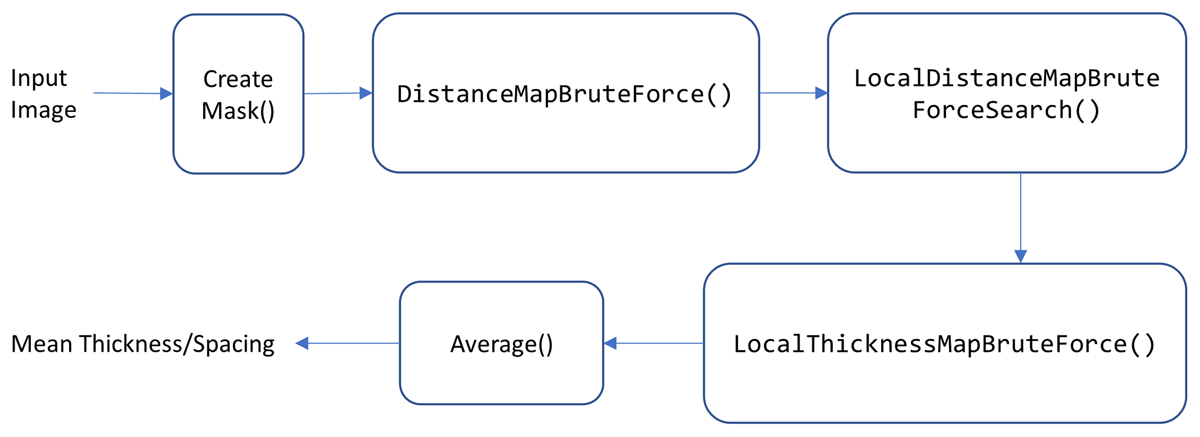
Figure 4
Workflows of the brute force algorithm.
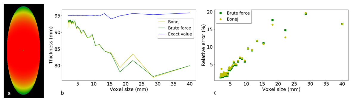
Figure 5
Accuracy of thickness computations on ellipsoid. a) Slice through the analytically derived local thickness map of the ellipsoid with diameters 100 × 100 × 300 mm3. The red color has a higher intensity, corresponding to a bigger local thickness. b) Mean local thickness as a function of voxel size in comparison with the exact values, which were mathematically calculated per voxel. Coarse voxels cause an underestimation of the thickness. c) The relative error to the exact value increases with the voxel size. BoneJ and the brute force algorithm have similar relative errors which increase with the growth of the voxel size.
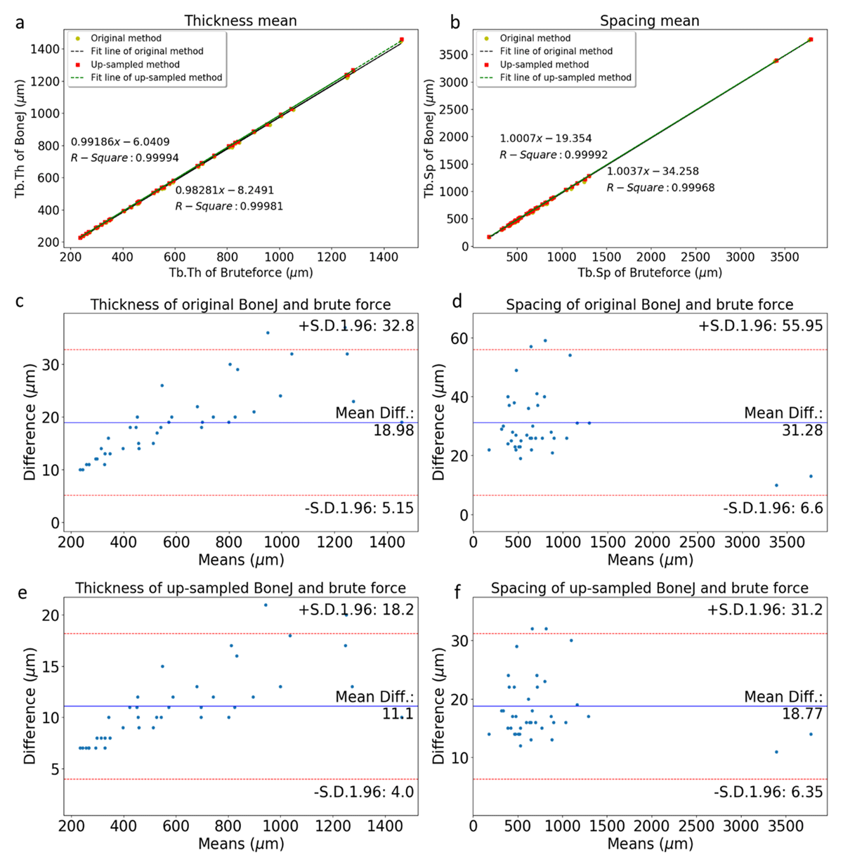
Figure 6
Comparison between brute force and BoneJ for 40 bone datasets. Strong correlation between brute force and BoneJ appears for trabecular thickness (a) and trabecular spacing (b), with and without upsampling. Bland-Altman plots for trabecular thickness (c) and trabecular spacing (d) show systematically lower values for BoneJ compared to brute force, on the order of the voxel size. Bland-Altman plots for upsampled results (e, f) show stronger agreement between BoneJ and brute force.
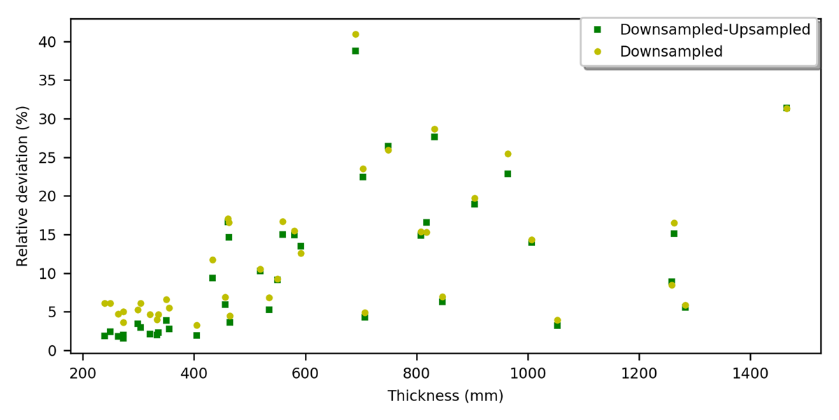
Figure 7
Relative deviation of thicknesses of downsampled bone images and downsampled-upsampled bone images from those of the original images by the brute force method.