
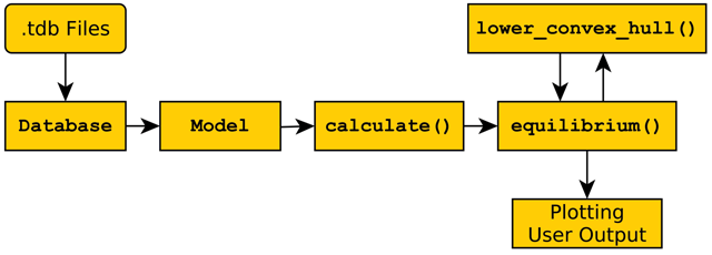
Figure 1
General architecture of the pycalphad software package. Using parameters from the given Database, a Model object is constructed for each phase and then fed into the calculation engine to produce results for the user.
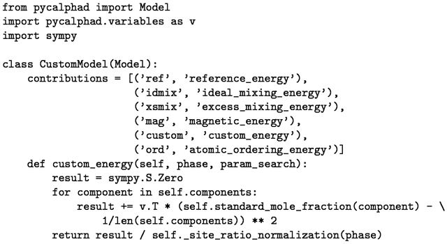
Figure 2
Creating a custom model in pycalphad involves creating a subclass of the Model class. The key step is declaring the contributions class attribute. The CustomModel subclass can then be passed as an argument to calculate() and equilibrium().
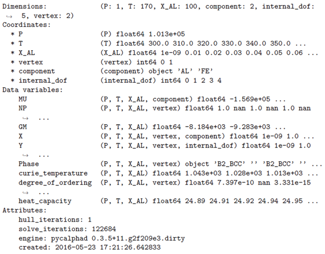
Figure 3
This is a summary of the result object returned by a call to equilibrium() when performing a 2-D mapping calculation. The “Dimensions” line indicates the shape of the array, with each dimension having a label and corresponding size. In this case, equilibria at 170 temperatures and 100 compositions are computed for a two component system. The “internal dof” dimension corresponds to the site fractions of a phase. The “vertex” dimension corresponds to the vertices of a tie simplex (tie-line in binary systems). The “Data Variables” section contains the actual result of the calculation, with the corresponding dimensions of each property array listed in parentheses, followed by the rst few values. The “Attributes” section contains some metadata about the calculation.
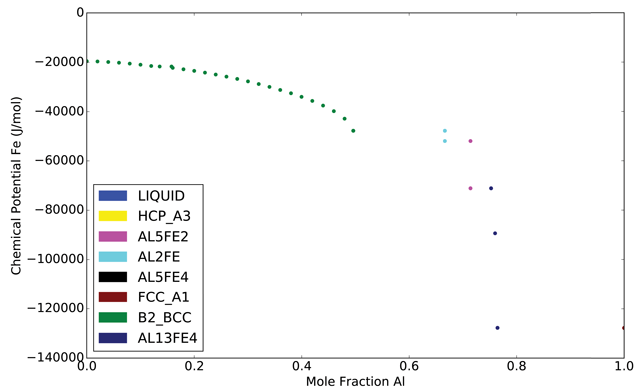
Figure 4
Equilibrium chemical potential of Fe as a function of Al composition in the Al-Fe system at 600 K, computed using pycalphad. Each point is color-coded with the corresponding stable phase; coexistence regions can be identied by the chemical potential remaining at across a range of composition. The end-points of such an iso-potential region can be directly connected to the corresponding tie-line at the given temperature.
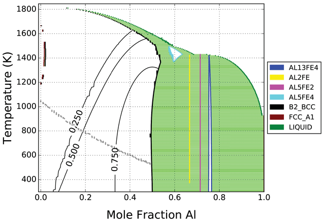
Figure 5
Phase diagram of the Al-Fe system according to the COST 507 database, computed using pycalphad. The solid black lines in the B2 region correspond to lines of constant “degree of ordering” in the B2 phase. The grey dashed line is the Curie temperature. The bcc ordering transition is second-order since the degree of ordering is continuously changing with respect to composition and temperature. Some lines in the diagram are not smooth due to the coarseness of the grid used in the calculation; mapping in pycalphad is still experimental.
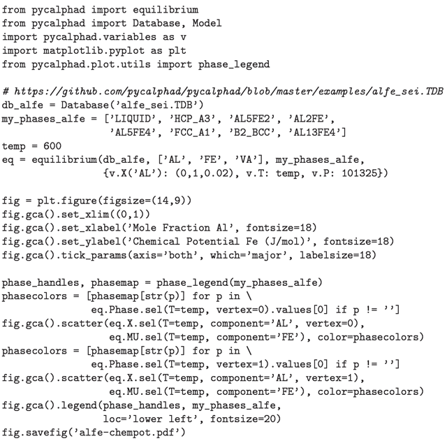
Figure 6
Source code for the Al-Fe chemical potential calculation in Figure 4.
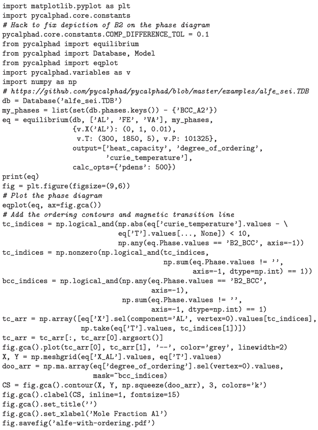
Figure 7
Source code for the Al-Fe phase diagram in Figure 5.