
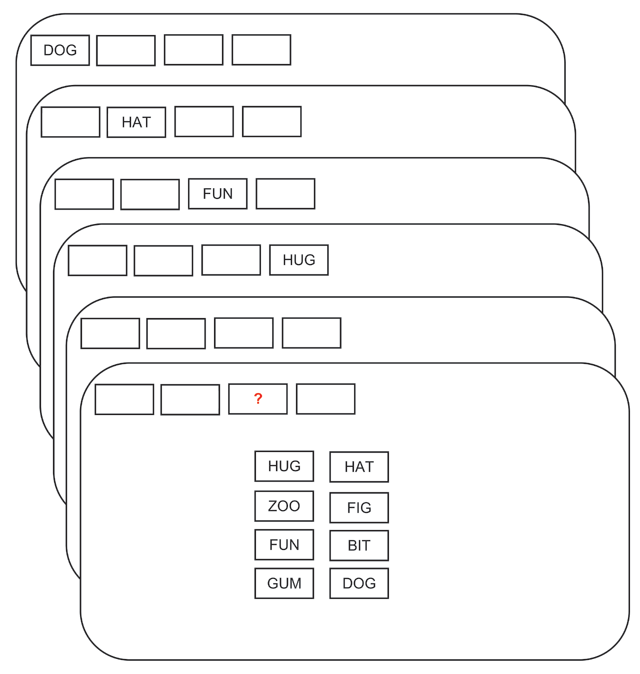
Figure 1
Flow of events in a trial with memory set size 4 and RSS = [4,4].
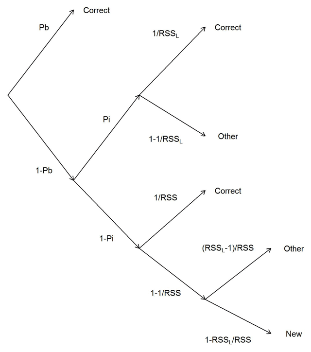
Figure 2
Structure of the multinomial process tree (MPT) model; at the end of each branch is the predicted response category (correct, other list word, or new word). Pb is the probability of remembering the target’s item-position binding; Pi is the probability of remembering which items have been in the current memory list. RSSL refers to the size of the subset of the response set that consists of current list items; RSS refers to the total size of the response set.
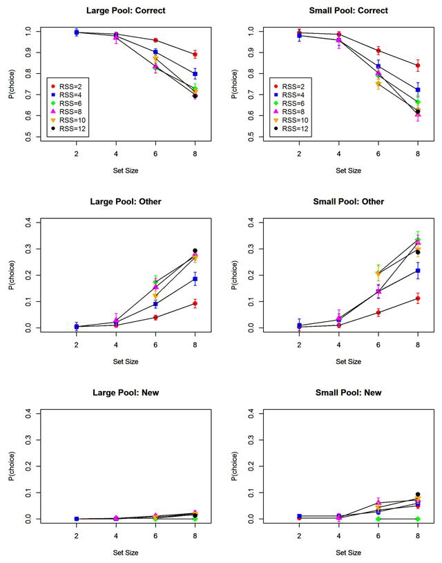
Figure 3
Proportion of correct responses, of responses selecting another than the correct list word, and of responses selecting a new word. Separate lines represent different response set sizes. Error bars are 95% confidence intervals corrected for within-subjects comparisons (Bakeman & McArthur, 1996).
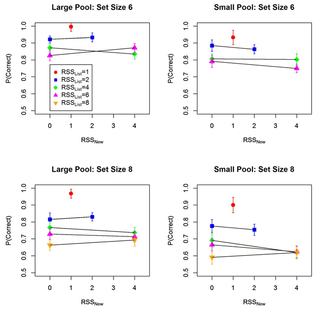
Figure 4
Proportion of correct responses as a function of memory set size (6 vs. 8), as well as the size of the response subset consisting of list words (RSSList) and the response subset consisting of new words (RSSNew). Error bars are 95% confidence intervals corrected for within-subjects comparisons (Bakeman & McArthur, 1996).
Table 1
Bayes Factors for Logistic Models.
| Memory Set Size | Response Set Size List | Response Set Size New | |
|---|---|---|---|
| Large-Pool Experiment | 1.07 × 10¹⁰ [1.00–1.77 × 10¹⁰] | 1.85 × 10¹¹ [1.16–3.36 × 10¹¹] | 0.37 [0.048–0.49] |
| Small-Pool Experiment | 4.14 × 10¹⁰ [3.29–7.21 × 10¹⁰] | 2.65 × 10⁸ [0.78–2.69 × 10⁸] | 14.2 [1.8–16.4] |
[i] Note: The Bayes factor reflects the strength of evidence for keeping the effect in question in the model over excluding it. It expresses the factor by which we should multiply the ratio of our prior probabilities assigned to the competing models to obtain our ratio of posterior probabilities. Bayes Factors are based on Cauchy priors on standardized effect sizes with a scale of .353; the range of Bayes Factors for scales between 0.25 and 3.0 obtained from the sensitivity analysis is given in brackets.
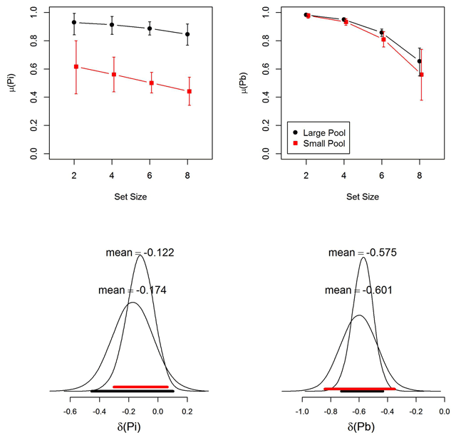
Figure 5
Top panels: Group-level parameter estimates (means of the posterior distribution) for item memory (Pi) and binding memory (Pb) from the MPT model. Black markers represent the large-pool experiment; red markers the small-pool experiment. Error bars are 95% highest-density intervals of the posteriors (Kruschke, 2011). Bottom panels: Posterior distribution of the slope of the linear effect of (mean-centered) memory set size on group means of Pi and Pb. Broad horizontal bars depict the 95% highest-density intervals (black for the large-pool experiment; red for the small-pool experiment).
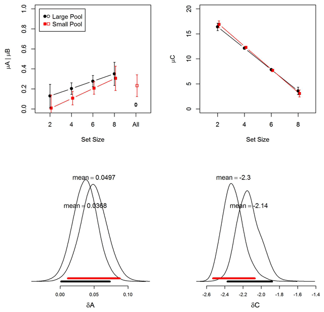
Figure 6
Top panels: Group-level parameter estimates (means of the posterior distribution) for item memory (A) and binding memory (C) from the memory measurement model (MMM). The upper-left panel also shows the B parameter, which was the same for all set sizes (“All” on the x-axis). Black markers represent the large-pool experiment; red markers the small-pool experiment. Error bars are 95% highest-density intervals of the posteriors (Kruschke, 2011). Bottom panels: Posterior distribution of the slope of the linear effect of (mean-centered) memory set size on group means of A and C. Broad horizontal bars depict the 95% highest-density intervals (black for the large-pool experiment; red for the small-pool experiment).
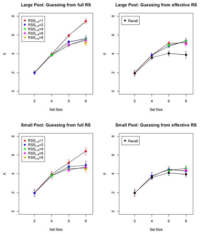
Figure 7
Estimates of capacity (K) on the assumption of discrete-state memory. The left panels show K estimates for a capacity limit on item memory; the right panels show K estimates for a capacity limit on binding memory. All panels show estimates from n-AFC tests as a function of the size of the response subset consisting of list words (RSSList); the right panels additionally show estimates from the recall test. Error bars are 95% confidence intervals corrected for within-subjects comparisons (Bakeman & McArthur, 1996).