
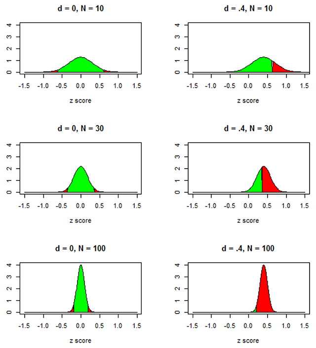
Figure 1
What happens to the significance of an effect when a study becomes more powerful? Red areas are p < .05, two-tailed t-test; green area is not significant.
Table 1
The outcome in terms of p-values a researcher can expect as a function of the effect size at the population level (no effect, effect of d = .4) and the number of participants tested in a two-tailed test. The outcome remains the same for the sample sizes when there is no effect at the population level, but it shifts towards smaller p-values in line with the hypothesis when there is an effect at the population level. For N = 10, the statistical test will be significant at p < .05 in 15 + 7 + 2 = 24% of the studies (so, this study has a power of 24%). For N = 30, the test will be significant in 24 + 21 + 14 = 49% of the studies. For N = 100, the test will be significant for 6 + 16 + 76 = 98% of the studies, of which the majority with have significance at p < .001. At the same time, even for this overpowered study researchers have 7% chance of finding a p-value hovering around .05.
| N = 10 | N = 30 | N = 100 | ||||
|---|---|---|---|---|---|---|
| d = 0 | d = .4 | d = 0 | d = .4 | d = 0 | d = .4 | |
| p < .001 against hypothesis | 0.0005 | ≈0% | 0.0005 | ≈0% | 0.0005 | ≈0% |
| .001 ≤ p < .01 against hypothesis | 0.0045 | ≈0% | 0.0045 | ≈0% | 0.0045 | ≈0% |
| .01 ≤ p < .05 against hypothesis | 0.0200 | 0.0006 | 0.0200 | ≈0% | 0.0200 | ≈0% |
| .05 ≤ p < .10 against hypothesis | 0.0250 | 0.0012 | 0.0250 | 0.0142 | 0.0250 | ≈0% |
| p ≥ .10 against hypothesis | 0.4500 | 0.1011 | 0.4500 | 0.2783 | 0.4500 | ≈0% |
| p ≥ .10 in line with hypothesis | 0.4500 | 0.5451 | 0.4500 | 0.1162 | 0.4500 | 0.0092 |
| .05 ≤ p < .10 in line with hypothesis | 0.0250 | 0.1085 | 0.0250 | 0.2412 | 0.0250 | 0.0114 |
| .01 ≤ p < .05 in line with hypothesis | 0.0200 | 0.1486 | 0.0200 | 0.2412 | 0.0200 | 0.0565 |
| .001 ≤ p < .01 in line with hypothesis | 0.0045 | 0.0735 | 0.0045 | 0.2144 | 0.0045 | 0.1618 |
| p < .001 in line with hypothesis | 0.0005 | 0.0214 | 0.0005 | 0.1357 | 0.0005 | 0.7610 |
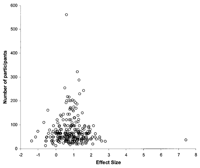
Figure 2
Tens of studies on the difference in vocabulary size between old and young adults. Positive effect sizes indicate that old adults know more words than young adults. Each circle represents a study. Circles at the bottom come from studies with few participants (about 20), studies at the top come from large studies (300 participants or more).
Source: Verhaeghen (2003).
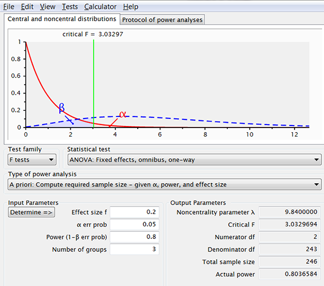
Figure 3
Output of G*Power when we ask the required sample sizes for f = .2 and three independent groups. This number is an underestimate because the f-value for a design with d = .4 between the extreme conditions and a smaller effect size for the in-between condition is slightly lower than f = .2. In addition, this is only the power of the omnibus ANOVA test with no guarantee that the population pattern will be observed in pairwise comparisons of the sample data.
Table 2
Example of data (reaction times) from a word recognition experiment as a function of prime type (related, unrelated).
| Participant | Related | Unrelated | Priming |
|---|---|---|---|
| p1 | 638 | 654 | 16 |
| p2 | 701 | 751 | 50 |
| p3 | 597 | 623 | 26 |
| p4 | 640 | 641 | 1 |
| p5 | 756 | 760 | 4 |
| p6 | 589 | 613 | 24 |
| p7 | 635 | 665 | 30 |
| p8 | 678 | 701 | 23 |
| p9 | 659 | 668 | 9 |
| p10 | 597 | 584 | –13 |
| Mean | 649 | 666 | 17 |
| Standard dev. | 52.2 | 57.2 | 17.7 |
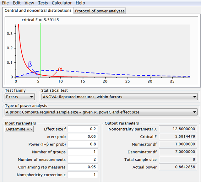
Figure 4
If one increases the correlation among the repeated measurements, G*Power indicates that fewer observations are needed. This is because G*Power takes the effect size to be dav, whereas the user often assumes it is dz.
Table 3
Correlations observed between the levels of a repeated-measures factor in a number of studies with different dependent variables.
| Study | Dependent variable | Correlation |
|---|---|---|
| Camerer et al. (2018) | ||
| Aviezer et al. (2012) | Valence ratings | –0.85 |
| Duncan et al. (2012) | Similarity identification | 0.89 |
| Kovacs et al. (2010) | Reaction time to visual stimuli | 0.84 |
| Sparrow et al. (2011) | Reaction time to visual stimuli | 0.81 |
| Zwaan et al. (2018) | ||
| associative priming | Reaction time to visual stimuli (Session 1) | 0.89 |
| Reaction time to visual stimuli (Session 2) | 0.93 | |
| false memories | Correct related-unrelated lures (Session 1) | –0.47 |
| Correct related-unrelated lures (Session 2) | –0.14 | |
| flanker task | RT stimulus congruent incongruent (Session 1) | 0.95 |
| RT stimulus congruent incongruent (Session 2) | 0.93 | |
| shape simulation | RT to shape matching sentence (Seesion 1) | 0.89 |
| RT to shape matching sentence (Seesion 2) | 0.92 | |
| spacing effect | Memory of massed v. spaced items (Session 1) | 0.35 |
| Memory of massed v. spaced items (Session 2) | 0.55 |
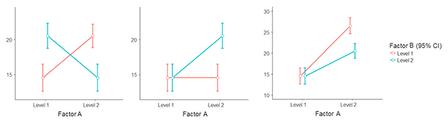
Figure 3
Different types of interactions researchers may be interested in. Left panel: fully crossed interaction. Middle panel: the effect of A is only present for one level of B. Right panel: The effect of A is very strong for one level of B and only half as strong for the other level.
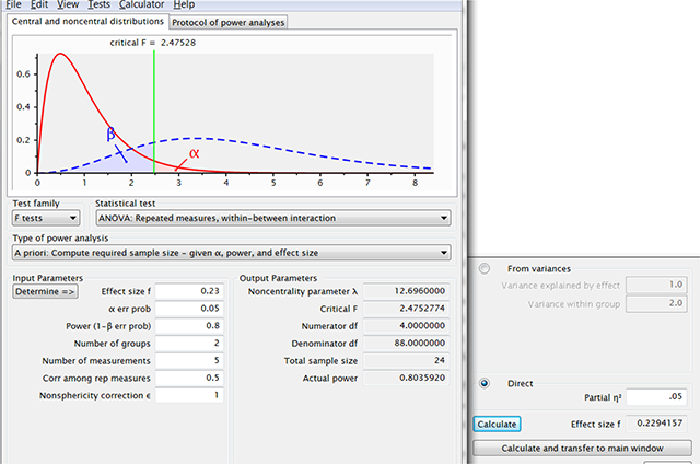
Figure 4
Figure illustrating how you can convince yourself with G*Power that two groups of 15 participants allow you to find effect sizes of f = .23 in a split-plot design with two groups and five levels of the repeated-measures variable. When seeing this type of output, it good to keep in mind that you need 50 participants for a typical effect in a t-test with related samples. This not only sounds too good to be true, it is also too good to be true.
Table 4
Responses of six participants (P1–P6) to four repetitions of the same stimulus (S1–S4).
| S1 | S2 | S3 | S4 | |
|---|---|---|---|---|
| P1 | 7 | 5 | 10 | 6 |
| P2 | 9 | 11 | 8 | 10 |
| P3 | 12 | 9 | 17 | 14 |
| P4 | 11 | 8 | 6 | 18 |
| P5 | 7 | 3 | 3 | 6 |
| P6 | 10 | 14 | 7 | 14 |
Table 5
First lines of the long notation of Table 4. Lines with missing values are simply left out.
| Participant | Condition | Response |
|---|---|---|
| P1 | S1 | 7 |
| P1 | S2 | 5 |
| P1 | S3 | 10 |
| P1 | S4 | 6 |
| P2 | S1 | 9 |
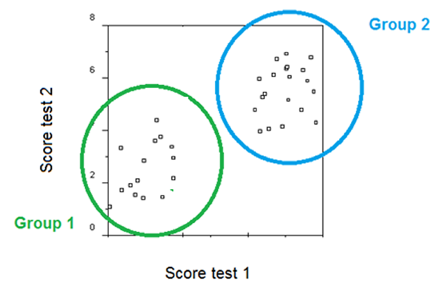
Figure 5
Illustration of how you can find a high correlation in the entire dataset (because of the group difference) and a low correlation within each group (because of the range restriction within groups).
Table 5
Intraclass correlations for designs with one repeated-measures factor (2 levels). The experiments of Zwaan et al. included more variables, but these did not affect the results much, so that the design could be reduced to a one-way design. The table shows the intraclass correlations, which mostly reach the desired level of ICC2 = .80 when it is calculated within conditions. The table also shows that the average reported effect size was dz = .76. If the experiments had been based on a single observation per condition, the average effect size would have been dz = .24, illustrating the gain that can be made by having multiple observations per participant per condition.
| Study | Dependent variable | N parts | N conditions | Nobs_per_ cond | Across the entire dataset | Average within condition | dN = 1 | dN = tot | ||
|---|---|---|---|---|---|---|---|---|---|---|
| ICC1 | ICC2 | ICC1 | ICC2 | |||||||
| Camerer et al. (2018) | ||||||||||
| Aviezer et al. (2012) | Valence ratings | 14 | 2 | 88 | 0.01 | 0.60 | 0.23 | 0.96 | 0.94 | 1.43 |
| Kovacs et al. (2010) | Reaction time to visual stimuli | 95 | 2 | 5 | 0.41 | 0.87 | 0.40 | 0.76 | 0.29 | 0.72 |
| Sparrow et al. (2011) | Reaction time to visual stimuli | 234 | 2 | 8 & 16 | 0.10 | 0.91 | 0.10 | 0.81 | 0.03 | 0.10 |
| Zwaan et al. (2018) | ||||||||||
| associative priming | Reaction time to visual stimuli (Session 1) | 160 | 2 × 2 × 2 | 30 | 0.28 | 0.96 | 0.31 | 0.93 | 0.17 | 0.81 |
| Reaction time to visual stimuli (Session 2) | 0.30 | 0.96 | 0.31 | 0.92 | 0.18 | 0.94 | ||||
| false memories | Correct related-unrelated lures (Session 1) | 160 | 2 × 2 × 2 | 9 | 0.02 | 0.29 | 0.27 | 0.77 | 0.20 | 0.97 |
| Correct related-unrelated lures (Session 2) | 0.06 | 0.54 | 0.26 | 0.75 | 0.31 | 1.17 | ||||
| flanker task | RT stimulus congruent incongruent (Session 1) | 160 | 2 × 2 × 2 | 32 | 0.40 | 0.98 | 0.41 | 0.96 | 0.15 | 0.70 |
| RT stimulus congruent incongruent (Session 2) | 0.29 | 0.96 | 0.29 | 0.92 | 0.13 | 0.52 | ||||
| shape simulation | RT to shape matching sentence (Seesion 1) | 160 | 2 × 2 × 2 | 15 | 0.42 | 0.93 | 0.42 | 0.91 | 0.08 | 0.27 |
| RT to shape matching sentence (Seesion 2) | 0.49 | 0.97 | 0.50 | 0.94 | 0.17 | 0.50 | ||||
| spacing effect | Memory of massed v. spaced items (Session 1) | 160 | 2 × 2 × 2 | 40 | 0.03 | 0.54 | 0.03 | 0.40 | 0.20 | 0.87 |
| Memory of massed v. spaced items (Session 1) | 0.06 | 0.84 | 0.07 | 0.75 | 0.21 | 0.92 | ||||
Table 6
Intraclass correlations for between-groups designs. The table shows that the intraclass correlations mostly reached the desired level of ICC2 = .80 when multiple observations were made per condition and all the items used. In general, this improved the interpretation (see in particular the study of Pyc & Rawson, 2010). At the same time, for some dependent variable (e.g., rating scales) rather stable data can be obtained with a few questions (see the study by Wilson et al., 2014).
| Study | Dependent variable | N parts | N conditions | Nobs_per_ cond | Across the entire dataset | Average within condition | dN = 1 | dN = tot | ||
|---|---|---|---|---|---|---|---|---|---|---|
| ICC1 | ICC2 | ICC1 | ICC2 | |||||||
| Camerer et al. (2018) | ||||||||||
| Ackerman et al. (2010) | Evaluating job candicates | 599 | 2 | 8 | 0.47 | 0.87 | 0.47 | 0.88 | 0.10 | 0.13 |
| Gervais & Norenzayan (2012) | Belief in God | 531 | 2 | 1 | NA | NA | NA | NA | –0.07 | –0.07 |
| Karpicke & Blunt (2011) | Text memory | 49 | 2 | 1 | NA | NA | NA | NA | 0.83 | 0.83 |
| Kidd & Castano (2013) | Emotion recognition | 714 | 2 | 36 | 0.09 | 0.78 | 0.09 | 0.78 | –0.03 | –0.08 |
| Morewedge et al. (2010) | M&Ms eaten | 89 | 2 | 1 | NA | NA | NA | NA | 0.75 | 0.75 |
| Pyc & Rawson (2010) | Word translations | 306 | 2 | 48 | 0.14 | 0.89 | 0.14 | 0.88 | 0.12 | 0.30 |
| Shah et al (2012) | Dots-mixed task | 619 | 2 | 1 | NA | NA | NA | NA | –0.03 | –0.03 |
| Wilson et al (2014) | Enjoyment ratings | 39 | 2 | 3 | 0.82 | 0.93 | 0.73 | 0.89 | 1.32 | 1.44 |
Table 7
Numbers of participants required for various designs when d = .4, .5, and .6 and the data are analyzed with traditional, frequentist statistics (p < .05). The numbers of the d = .4 column are the default numbers to use. The higher values of d require dependent variables with a reliability of .8 at least. Therefore, authors using these estimates must present evidence about the reliability of their variables. This can easily be done by calculating the ICC1 and ICC2 values discussed above.
| Traditional, frequentist analysis (p < .05) | |||
|---|---|---|---|
| d = .4 | d = .5 | d = .6 | |
| 1 variable between-groups | |||
| • 2 levels | 200 | 130 | 90 |
| • 2 levels, null hypothesis | 860 | 860 | 860 |
| • 3 levels (I = II > III) | 435 | 285 | 195 |
| • 3 levels (I > II > III) | 1740 | 1125 | 795 |
| 1 variable within-groups | |||
| • 2 levels | 52 | 34 | 24 |
| • 2 levels, null hypothesis | 215 | 215 | 215 |
| • 3 levels (I = II > III) | 75 | 50 | 35 |
| • 3 levels (I > II > III) | 300 | 195 | 130 |
| Correlation | 195 | 125 | 85 |
| 2 × 2 repeated measures | |||
| • Main effect one variable | 27 | 18 | 13 |
| • Interaction (d v. 0) | 110 | 75 | 50 |
| 2 × 2 split-plot | |||
| • Main effect between | |||
| ◦ r = .5 | 150 | 100 | 70 |
| ◦ r = .9 | 190 | 120 | 90 |
| • Main effect repeated-measure | 55 | 34 | 24 |
| • Interaction (d v. 0) | 200 | 130 | 90 |
| • ANCOVA | |||
| ◦ rrep_measure = .5 | 160 | 100 | 70 |
| ◦ rrep_measure = .9 | 200 | 130 | 90 |
Table 8
Numbers of participants required for various designs when d = .4, .5, and .6 and the data are analyzed with Bayesian statistics (BF > 10). The numbers of the d = .4 column are the default numbers to use. The higher values of d require dependent variables with a reliability of .8 at least. Therefore, authors using these estimates must present evidence about the reliability of their variables. This can easily be done by calculating the ICC1 and ICC2 values discussed above.
| Bayesian analysis (BF > 10) | |||
|---|---|---|---|
| d = .4 | d = .5 | d = .6 | |
| 1 variable between-groups | |||
| • 2 levels | 380 | 240 | 170 |
| • 2 levels, null hypothesis | 2400 | 2400 | 2400 |
| • 3 levels (I = II > III) | 690 | 450 | 300 |
| • 3 levels (I > II > III) | 2850 | 1800 | 1200 |
| 1 variable within-groups | |||
| • 2 levels | 100 | 65 | 45 |
| • 2 levels, null hypothesis | 720 | 720 | 720 |
| • 3 levels (I = II > III) | 125 | 80 | 55 |
| • 3 levels (I > II > III) | 540 | 340 | 240 |
| Correlation | 370 | 230 | 160 |
| 2 × 2 repeated measures | |||
| • Main effect one variable | 52 | 32 | 23 |
| • Interaction (d v. 0) | 210 | 130 | 85 |
| 2 × 2 split-plot | |||
| • Main effect between | |||
| ◦ r = .5 | 290 | 190 | 130 |
| ◦ r = .9 | 360 | 220 | 160 |
| • Main effect repeated-measure | 100 | 66 | 46 |
| • Interaction (d v. 0) | 390 | 250 | 170 |
| • ANCOVA | |||
| ◦ rrep_measure = .5 | 300 | 190 | 130 |
| ◦ rrep_measure = .9 | 380 | 230 | 170 |
Table 9
Numbers of participants required for various designs when d = .4 and power is increased to 90%. The latter decreases the chances of not finding an effect present in the population.
| d = .4, power = .9, p < .05 | d = .4, power = .9, BF > 10 | |
|---|---|---|
| 1 variable between-groups | ||
| • 2 levels | 264 | 480 |
| • 2 levels, null hypothesis | 1084 | 3600 |
| • 3 levels (I = II > III) | 570 | 840 |
| • 3 levels (I > II > III) | 2160 | 3450 |
| 1 variable within-groups | ||
| • 2 levels | 70 | 130 |
| • 2 levels, null hypothesis | 271 | 1800 |
| • 3 levels (I = II > III) | 100 | 150 |
| • 3 levels (I > II > III) | 360 | 610 |
| Correlation | 260 | 460 |
| 2 × 2 repeated measures | ||
| • Main effect one variable | 35 | 65 |
| • Interaction (d v. 0) | 145 | 270 |
| 2 × 2 split-plot | ||
| • Main effect between | ||
| ◦ r = .5 | 200 | 360 |
| ◦ r = .9 | 250 | 450 |
| • Main effect repeated-measure | 70 | 130 |
| • Interaction (d v. 0) | 300 | 540 |
| • ANCOVA | ||
| ◦ rrep_measure = .5 | 210 | 360 |
| ◦ rrep_measure = .9 | 260 | 460 |
Table 10
Comparison of dz and dav for repeated-measures designs in Zwaan et al. (2018). They show that dav < dz when r = .5 (see Table 3). Reporting dav in addition to dz for pairwise comparisons allows readers to compare the effect sizes of repeated-measures studies with those of between-groups studies.
| Study | Dependent variable | N parts | N conditions | Nobs_ per_cond | dzN=1 | dzN = tot | dav |
|---|---|---|---|---|---|---|---|
| Zwaan et al. (2018) | |||||||
| associative priming | Reaction time to visual stimuli (Session 1) | 160 | 2 × 2 × 2 | 30 | 0.17 | 0.81 | 0.37 |
| Reaction time to visual stimuli (Session 2) | 0.18 | 0.94 | 0.35 | ||||
| false memories | Correct related-unrelated lures (Session 1) | 160 | 2 × 2 × 2 | 9 | 0.20 | 0.97 | 1.66 |
| Correct related-unrelated lures (Session 2) | 0.31 | 1.17 | 1.76 | ||||
| flanker task | RT stimulus congruent incongruent (Session 1) | 160 | 2 × 2 × 2 | 32 | 0.15 | 0.70 | 0.44 |
| RT stimulus congruent incongruent (Session 2) | 0.13 | 0.52 | 0.20 | ||||
| shape simulation | RT to shape matching sentence (Seesion 1) | 160 | 2 × 2 × 2 | 15 | 0.08 | 0.27 | 0.13 |
| RT to shape matching sentence (Seesion 2) | 0.17 | 0.50 | 0.21 | ||||
| spacing effect | Memory of massed v. spaced items (Session 1) | 160 | 2 × 2 × 2 | 40 | 0.20 | 0.87 | 1.00 |
| Memory of massed v. spaced items (Session 2) | 0.21 | 0.92 | 0.87 | ||||