
Table 1
Mapping model predictions to theoretical constructs.
| ACCOUNT | DESCRIPTION | LOCI | CONTRAST | EX-GAUSSIAN PREDICTIONS | QUANTILE PLOTS | RECOGNITION MEMORY PREDICTIONS |
|---|---|---|---|---|---|---|
| Meta-cognitive | Perceptual disfluency affects meta-cognitive processes via increased system 2 processing | Post-lexical | High-blur vs. Low-blur/Clear | μ: × β/τ: ↑ | Late difference | High > Low/Clear |
| Low-blur vs. Clear | μ: × β/τ: ↑ | Late difference | Low > Clear | |||
| Compensatory-processing | Perceptual disfluency affects word recognition | Lexical/semantic | High-blur vs. Low-blur/Clear | μ: ↑ β/τ: × | Complete shift | High > Low/Clear |
| Low-blur vs. Clear | μ: × β/τ: × | No difference | Low = Clear | |||
| Stage-specific | Disfluency effects rely on (1) the stage or level of processing tapped by the task and (2) monitoring and control processes | Lexical/semantic and Post-lexical | High-blur vs. Low-blur/Clear | μ: ↑ β/τ: ↑ | Complete shift Shift + Late differences | High > Low/Clear |
| Low-blur vs. Clear | μ: ↑ β/τ: × | No difference | Low = Clear |
[i] Note. ↑ = higher estimate; ↓ = decrease estimate; x = no effect on parameter of interest.

Figure 1
Clear (left), low-blur (10% blur) (right), and high-blur (15% blur) (center) examples.
Table 2
Posterior distribution estimates for accuracy model (Experiments 1A and 1B).
| EXPERIMENT | HYPOTHESIS | MEAN | SE | CrI* | ER | POSTERIOR PROB |
|---|---|---|---|---|---|---|
| Experiment 1A | High-blur < (Low-blur + Clear) | –1.03 | 0.16 | [–1.293, –0.77] | Inf | 1.00 |
| Low-blur < Clear | 0.04 | 0.13 | [–0.216, 0.297] | 1.26 | 0.56 | |
| Experiment 1B | High-blur < (Low-blur + Clear) | –1.10 | 0.17 | [–1.376, –0.829] | Inf | 1.00 |
| Low-blur = Clear | 0.03 | 0.15 | [–0.278, 0.322] | 0.90 | 0.47 |
[i] Note. CrI: 90% for one-sided tests and 95% for two-sided tests against 0. Posterior probability indicates the proportion of the posterior distribution that falls on one side of zero (either positive or negative), representing the probability that the effect is greater than or less than zero.
Table 3
Posterior distribution estimates for ex-Gaussian distribution (Experiments 1A and 1B).
| EXPERIMENT | HYPOTHESIS | PARAMETER | MEAN | SE | CrI* | ER | POSTERIOR PROB |
|---|---|---|---|---|---|---|---|
| Experiment 1A | High-blur > (Low-blur + Clear) | Mu (µ) | 0.11 | 0.00 | [0.1, 0.114] | Inf | 1.00 |
| Experiment 1B | High-blur > (Low-blur + Clear) | Mu (µ) | 0.12 | 0.01 | [0.11, 0.127] | Inf | 1.00 |
| Experiment 1A | High-blur > (Low-blur + Clear) | Sigma (σ) | 0.16 | 0.06 | [0.057, 0.253] | 163.95 | 0.99 |
| Experiment 1B | High-blur > (Low-blur + Clear) | Sigma (σ) | 0.32 | 0.07 | [0.214, 0.43] | Inf | 1.00 |
| Experiment 1A | High-blur > (Low-blur + Clear) | Beta (β/τ) | 0.43 | 0.04 | [0.367, 0.487] | Inf | 1.00 |
| Experiment 1B | High-blur > (Low-blur + Clear) | Beta (β/τ) | 0.38 | 0.03 | [0.318, 0.43] | Inf | 1.00 |
| Experiment 1A | Low-blur = Clear | Sigma (σ) | 0.03 | 0.05 | [–0.066, 0.136] | 16.22 | 0.94 |
| Experiment 1B | Low-blur = Clear | Sigma (σ) | –0.09 | 0.06 | [–0.212, 0.035] | 5.92 | 0.85 |
| Experiment 1A | Low-blur = Clear | Beta (β/τ) | –0.00 | 0.03 | [–0.062, 0.061] | 7.77 | 0.89 |
| Experiment 1B | Low-blur = Clear | Beta (β/τ) | 0.03 | 0.03 | [–0.026, 0.084] | 5.05 | 0.83 |
| Experiment 1A | Low-blur > Clear | Mu (µ) | 0.02 | 0.00 | [0.012, 0.02] | Inf | 1.00 |
| Experiment 1B | Low-blur > Clear | Mu (µ) | 0.01 | 0.00 | [0.006, 0.015] | Inf | 1.00 |
[i] Note. CrI: 90% for one-sided tests and 95% for two-sided tests against 0. Posterior probability indicates the proportion of the posterior distribution that falls on one side of zero (either positive or negative), representing the probability that the effect is greater than or less than zero.
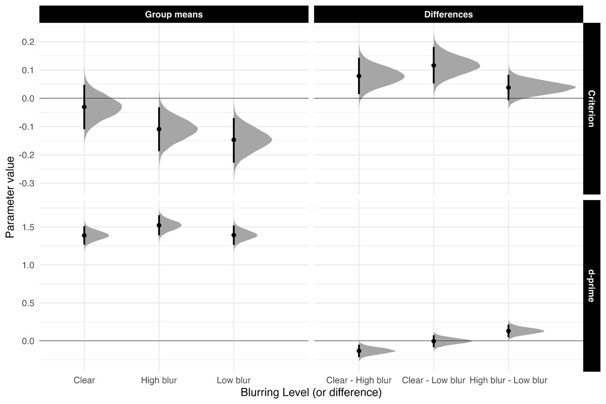
Figure 2
Estimated posterior distributions for d-prime and criterion, and differences, with 95% CrIs.
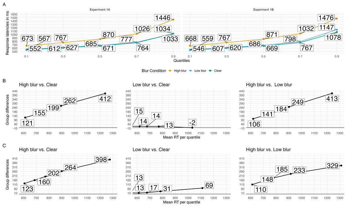
Figure 3
Quantile plots for each blur condition in Experiments 1A and 1B (A) and delta plots depicting the magnitude of the effect for hypotheses of interest over time in Experiments 1A (B) and 1B (C). Each dot represents the mean RT at the .1, .3, .5, .7 and .9 quantiles.
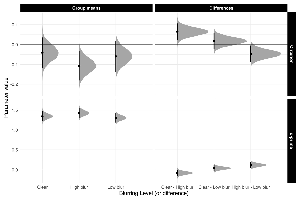
Figure 4
Estimated posterior distributions (mean) for d-prime and criterion, and differences, with 95% CrIs.
Table 4
Posterior distribution estimates for accuracy model (Experiment 2).
| HYPOTHESIS | MEAN | SE | CrI* | ER | POSTERIOR PROB |
|---|---|---|---|---|---|
| High-blur < (Low-blur + Clear) | –0.91 | 0.21 | [–1.263, –0.56] | Inf | 1.00 |
| Low-blur = Clear | –0.19 | 0.21 | [–0.628, 0.203] | 0.57 | 0.36 |
| High frequency = Low frequency | 0.15 | 0.20 | [–0.215, 0.548] | 0.67 | 0.40 |
| Blur × Frequency (High vs. Low/Clear) = 0 | –0.01 | 0.23 | [–0.47, 0.438] | 0.73 | 0.42 |
| Blur × Frequency (Low vs. Clear) = 0 | 0.05 | 0.24 | [–0.406, 0.554] | 0.72 | 0.42 |
[i] Note. CrI: 90% for one-sided tests and 95% for two-sided tests against 0. Posterior probability indicates the proportion of the posterior distribution that falls on one side of zero (either positive or negative), representing the probability that the effect is greater than or less than zero.
Table 5
Posterior distribution estimates for ex-Gaussian distribution (Experiment 2).
| HYPOTHESIS | PARAMETER | MEAN | SE | CrI* | ER | POSTERIOR PROB |
|---|---|---|---|---|---|---|
| high-blur > (vs. Clear/low-blur) | Mu (µ) | 0.17 | 0.01 | [0.164, 0.18] | Inf | 1.00 |
| low-blur > Clear | Mu (µ) | 0.01 | 0.00 | [0.008, 0.013] | Inf | 1.00 |
| High Frequency < Low frequency | Mu (µ) | –0.02 | 0.01 | [–0.026, –0.011] | Inf | 1.00 |
| High-blur (vs. Low-blur/Clear) × Frequency | Mu (µ) | –0.01 | 0.01 | [–0.02, 0.009] | 1,024.59 | 1.00 |
| Low-blur (vs. Clear) × Frequency | Mu (µ) | –0.00 | 0.00 | [–0.009, 0.002] | 1,453.96 | 1.00 |
| High-blur > (vs. Clear/low-blur) | Sigma (σ) | 0.64 | 0.04 | [0.562, 0.706] | Inf | 1.00 |
| Low-blur < Clear | Sigma (σ) | –0.01 | 0.03 | [–0.061, 0.045] | 1.41 | 0.58 |
| High frequency < Low frequency | Sigma (σ) | –0.05 | 0.04 | [–0.108, 0.01] | 11.05 | 0.92 |
| High-blur (vs. low-blur/Clear) × Frequency | Sigma (σ) | 0.08 | 0.07 | [–0.031, 0.197] | 7.67 | 0.89 |
| Low-blur (vs. Clear) × Frequency | Sigma (σ) | –0.03 | 0.06 | [–0.129, 0.065] | 2.31 | 0.70 |
| High-blur > (vs. Clear/low-blur) | Beta (β/τ) | 0.55 | 0.03 | [0.499, 0.603] | Inf | 1.00 |
| Low-blur > (vs. Clear) | Beta (β/τ) | –0.01 | 0.02 | [–0.055, 0.027] | 9.72 | 0.91 |
| High frequency < Low frequency | Beta (β/τ) | –0.07 | 0.03 | [–0.114, –0.016] | 67.18 | 0.98 |
| High-blur (vs. Low-blur/Clear) × Frequency | Beta (β/τ) | –0.14 | 0.05 | [–0.222, –0.056] | 332.33 | 1.00 |
| Low-blur (vs. Clear) × Frequency | Beta (β/τ) | 0.06 | 0.04 | [0, 0.129] | 19.52 | 0.95 |
[i] Note. CrI: 90% for one-sided tests and 95% for two-sided tests against 0. Posterior probability indicates the proportion of the posterior distribution that falls on one side of zero (either positive or negative), representing the probability that the effect is greater than or less than zero. Sigma and Beta parameters are on the log scale.
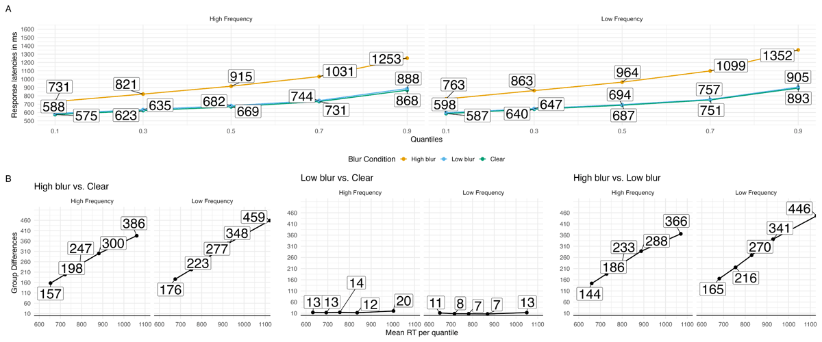
Figure 5
Group RT distributions in the blurring and word frequency manipulations in word stimuli. A. Quantile plots with each point represents the average RT quantiles (.1, .3, .5, .7, and .9) in each condition. B. Delta plots obtained by computing the quantiles for each participant and subsequently averaging the obtained values for each quantile over the participants and subtracting the values from each condition.
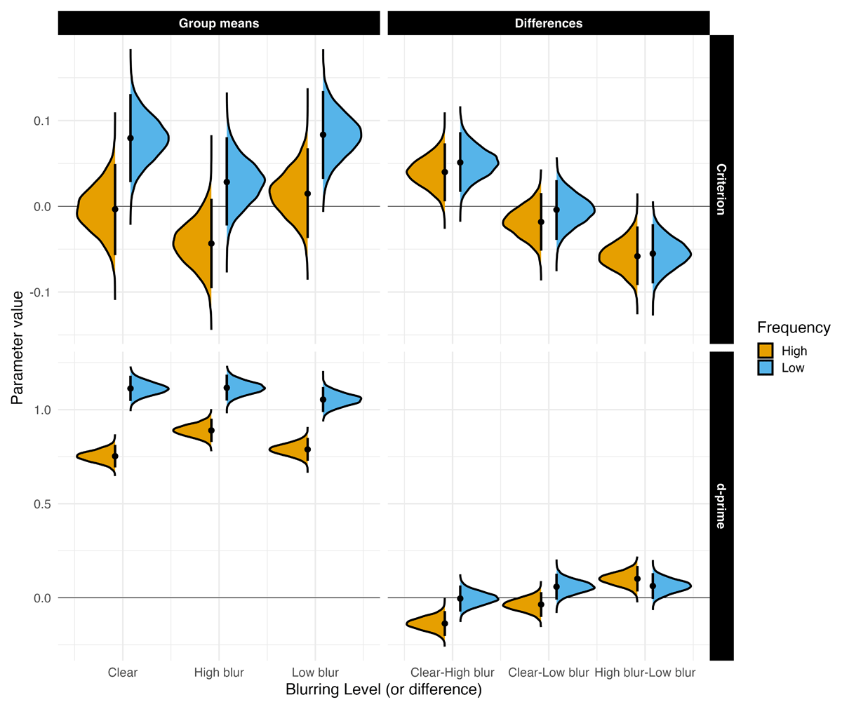
Figure 6
Estimated posterior distributions for d-prime and criterion, and differences between all conditions with 95% CrIs (thin lines).
Table 6
Mean response time (in ms) for the word frequency effects across the .1, .3, .5, .7, and .9 quantiles of the RT distribution as a function of blurring. These values correspond to the quantile effects for Experiment 2.
| BLUR | 0.1 | 0.3 | 0.5 | 0.7 | 0.9 |
|---|---|---|---|---|---|
| Clear | 12.10 | 17.17 | 18.59 | 19.24 | 25.06 |
| High-blur | 31.46 | 41.84 | 48.68 | 67.18 | 98.36 |
| Low-blur | 9.93 | 12.14 | 11.99 | 13.62 | 17.73 |
Table A1
Posterior distribution estimates for DDM (Experiment 1A).
| HYPOTHESIS | PARAMETER | MEAN | SE | CrI* | ER | POSTERIOR PROB |
|---|---|---|---|---|---|---|
| High-blur > (Low-blur + Clear) | v | –2.22 | 0.09 | [–2.369, –2.073] | Inf | 1.00 |
| low-blur = Clear | v | 0.00 | 0.05 | [–0.091, 0.096] | 29.65 | 0.97 |
| High-blur > (Low-blur + Clear) | Ter | 0.10 | 0.00 | [0.092, 0.106] | Inf | 1.00 |
| Low-blur > Clear | Ter | 0.01 | 0.00 | [0.008, 0.018] | Inf | 1.00 |
[i] Note. CrI: 90% for one-sided tests and 95% for two-sided tests against 0. Posterior probability indicates the proportion of the posterior distribution that falls on one side of zero (either positive or negative), representing the probability that the effect is greater than or less than zero.
Table A2
Posterior distribution estimates for DDM (Experiment 1B).
| HYPOTHESIS | PARAMETER | MEAN | SE | CrI* | ER | POSTERIOR PROB |
|---|---|---|---|---|---|---|
| High-blur < (low-blur + Clear) | v | –0.90 | 0.06 | [–1.001, –0.794] | Inf | 1.00 |
| Low-blur = Clear | v | –0.02 | 0.06 | [–0.13, 0.086] | 22.89 | 0.96 |
| High-blur > (Low-blur + Clear) | Ter | 0.10 | 0.01 | [0.093, 0.108] | Inf | 1.00 |
| Low-blur > Clear | Ter | 0.01 | 0.00 | [0.009, 0.02] | Inf | 1.00 |
[i] Note. CrI: 90% for one-sided tests and 95% for two-sided tests against 0. Posterior probability indicates the proportion of the posterior distribution that falls on one side of zero (either positive or negative), representing the probability that the effect is greater than or less than zero.