
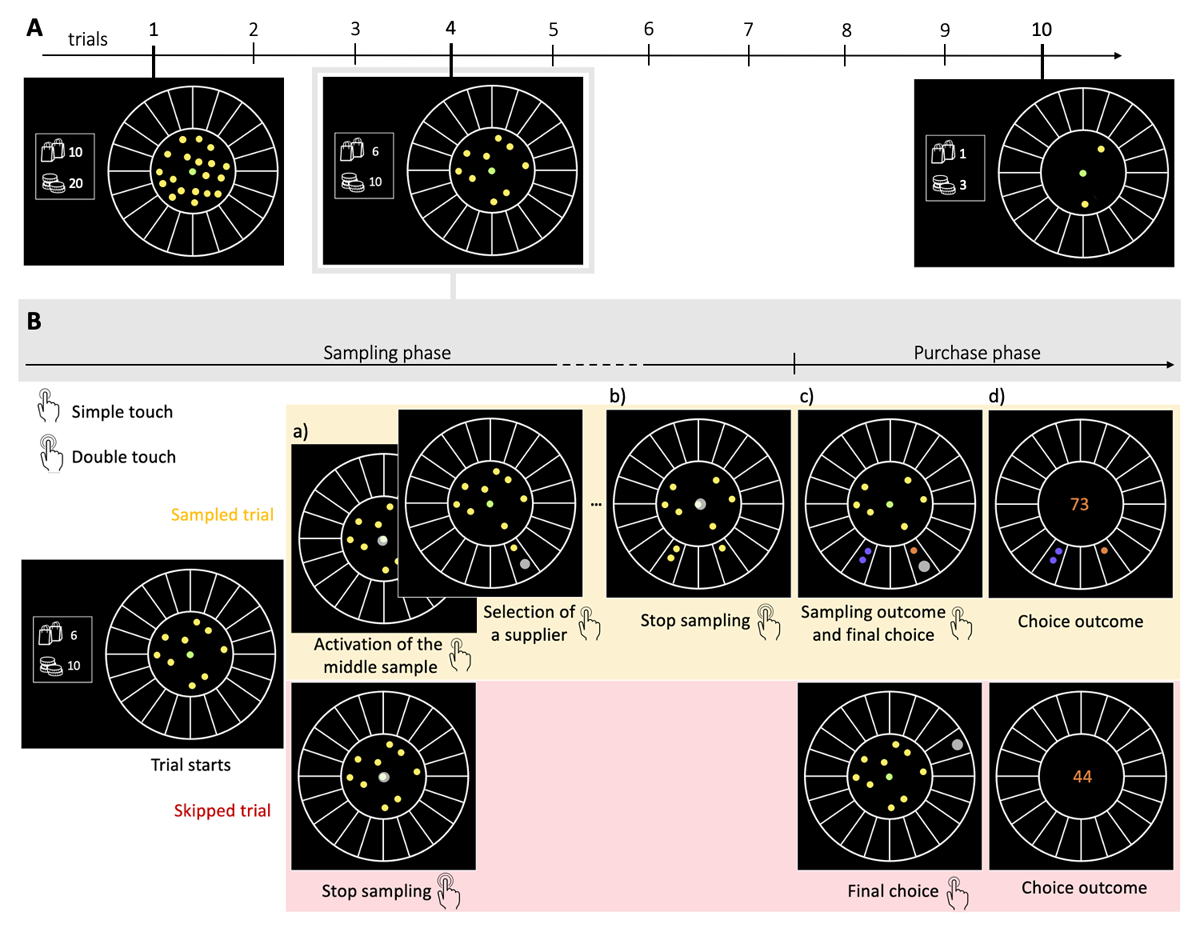
Figure 1
The BD apricot task with capacity freely allocated amongst trials. A. Example of one block composed of 10 consecutive choices (trials, Ntrials = 10) and with an initial capacity Nc of 20 samples. The capacity ratio r of this block represents the initial number of samples divided by the number of trials, in this case r = 2. On each trial, the remaining coins are displayed at any time in two ways: written on the left of the wheel (bottom number) and materialised by the yellow and green dots located within the centre of the wheel. For example, at the beginning of the 4th and last trial, the remaining capacity (Nr) is respectively of 10 and 3 samples. The remaining number of purchases (trials) in the block is also constantly displayed on the left of the wheel (top number). B. Example of one trial. Participants allocate a limited search capacity (coins) to assess the quality of good apricots in different suppliers (sampling phase). Subsequently, they make a final purchase of 100 apricots from one of the sampled suppliers (purchase phase). Each distinct black section of the wheel represents a different supplier. The initial number of coins per block varies pseudo-randomly from block to block within a finite range (defined by the capacity ratio r, multiplied by the number of trials in block Ntrials- see Methods). To allocate the coins to suppliers, participants have first to click on the designated active coin displayed at the centre (green dot) and then select the supplier to sample from (panels a) –both touch screen events are indicated by a large grey dot. One of the inactive (yellow) coins is then automatically activated and displayed, in green, at the centre. This sequence repeats until all coins are allocated or until participants end the sampling phase by touching twice the centre coin (panel b). Then, each of the allocated samples turn either orange, representing a good-quality apricot, or purple, representing a bad-quality apricot (panel c). Finally, after this information is revealed, the participant selects one of the sampled suppliers for the final purchase of 100 apricots (with a touch screen, indicated by a large grey dot) and the choice outcome is immediately displayed (panel d). In the case where no coin has been allocated (skipped trial – lower panels), participants select randomly one of the 20 suppliers for the final purchase.
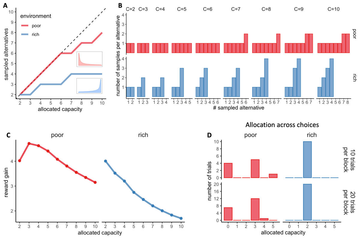
Figure 2
Optimal allocations of search capacity. A. Optimal BD trade-offs: number of alternatives sampled (M) maximising the expected reward depending on the capacity allocated in the trial and the environment richness (colours). Dashed lines indicate unit slope line. Prior distributions of success (proportion of good quality apricots) of each environment are plotted next to each curve. B. Number of samples allocated to each sampled alternative maximising the expected reward (optimal), depending on the capacity allocated C and the environment richness (colours). C. Reward gain (rg) as a function of the allocated capacity for each environment. rg is defined as rg = (𝔼[R│optimalmodel, C] – 𝔼[R│randommodel])/C, where R stands for the obtained reward. The reward gain is therefore the difference in reward expected when sampling with capacities from 2 to 10 (assuming an optimal BD trade-off) and when choosing randomly divided by the allocated capacity; such a quantity stresses the importance of following an optimal allocation strategy. D. Optimal distribution of trials depending on their sampling capacity, the block size and the environment richness for a capacity ratio r of 2.
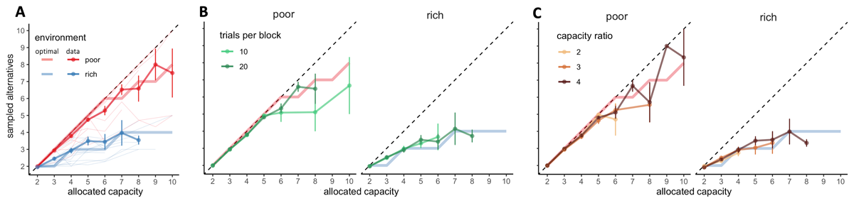
Figure 3
BD trade-offs are close-to-optimal and adapt to the environment, while being stable among blocks with different length and capacity ratio. A. Number of alternatives sampled (M) depending on the capacity allocated and the environment richness (colours). Group average and s.e.m. are plotted above individual data (thin light lines) and optimal values of M (thick light lines). Dashed lines indicate unit slope line. B-C. Colours represent the block length (B) or the capacity ratio r (C). N = 20 per environment.
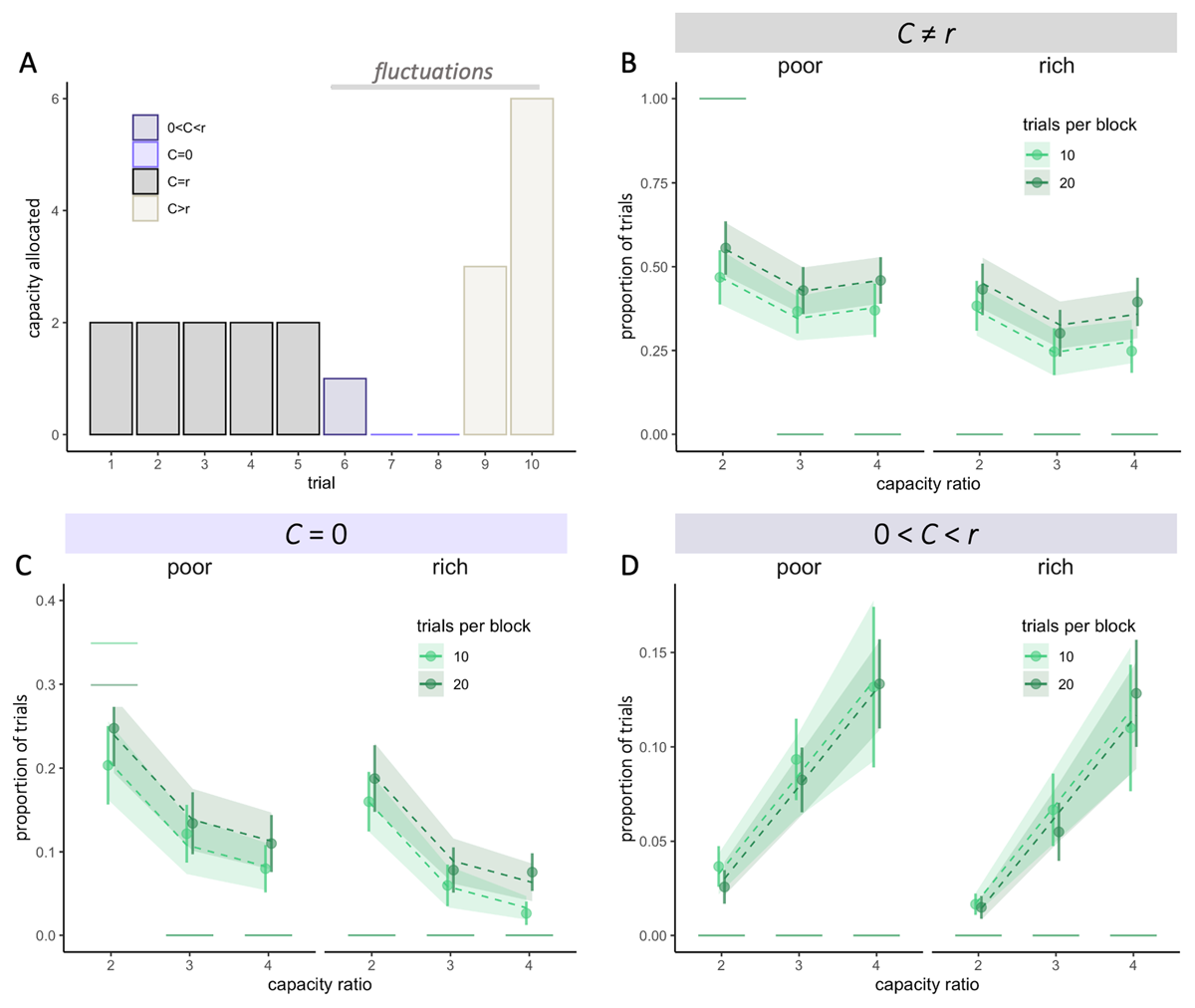
Figure 4
Participants capacity allocation fluctuates more when little capacity is available and with larger horizons. A. Example of capacity allocation (C) from one participant throughout consecutive trials in a block of length 10 and ratio r = 2. B-D. Fluctuations are defined as trials for which the allocated capacity C is different from r. Observed averaged proportions of trials (dots) where C ≠ r (fluctuations – B), C = 0 (skipped trials – C) and 0 < C < r (D), depending on the capacity ratio r, block length (colours) and the environment (poor or rich). Vertical bars represent s.e.m. of the data, while dashed lines and shaded areas represent respectively the predicted averages and s.e.m. using Linear Mixed Effect Models (LMEM). Horizontal segments represent the proportion of each type of trials predicted by the optimal model.
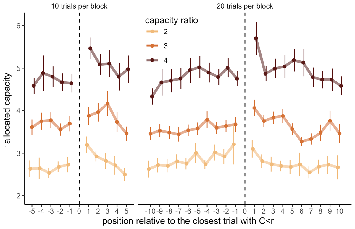
Figure 5
Allocating fewer capacity than the ratio is part of an anticipated strategy for sampling more in the next trial. Capacity allocated in trials depending on their relative position to the closest trial with an allocated capacity inferior to the capacity ratio of the block (C < r), depending on the block length (left: 10 trials, right: 20 trials) and the capacity ratio (colours). Each data point represents the average of 12 to 37 participants with at least 3 data points per participant. Vertical bars represent s.e.m.
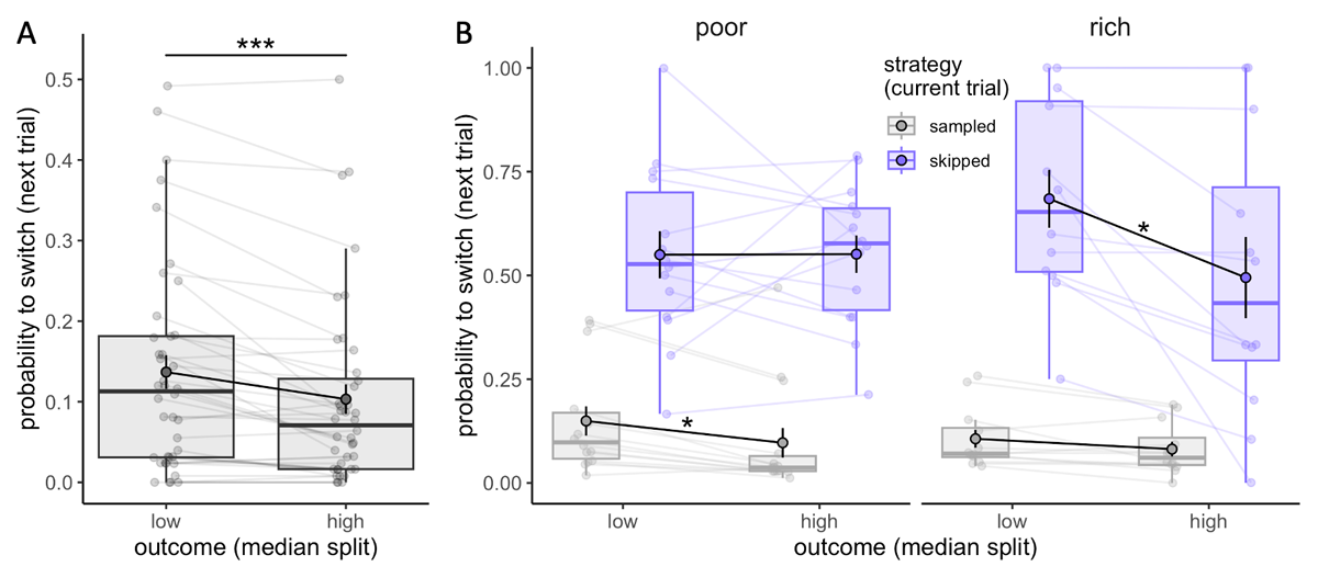
Figure 6
Participants adapt their sampling strategy to the outcome received. A-B. Probability to switch strategy in the next trial (from sampling to skipping and vice versa) depending on the outcome received (median split, calculated separately for individuals and skipped and sampled trials, N = 40) (A) and the strategy in the current trial (sampling or skipping) as well as the environment (poor: N = 14, rich: N = 12) (B). Boxplots represent the 1st and 3rd quartiles of the data distribution, with thicker horizontal black lines corresponding to medians and whiskers extended to the largest value no further than 1.5 times the inter-quartile range (IQR). Lighter dots represent individual data and are connected with lighter lines, while group averages are plotted on top (colour dots circled in black) and connected by black lines. Vertical black bars represent s.e.m. ‘*’: padj < .05, ‘***’: p < .001.
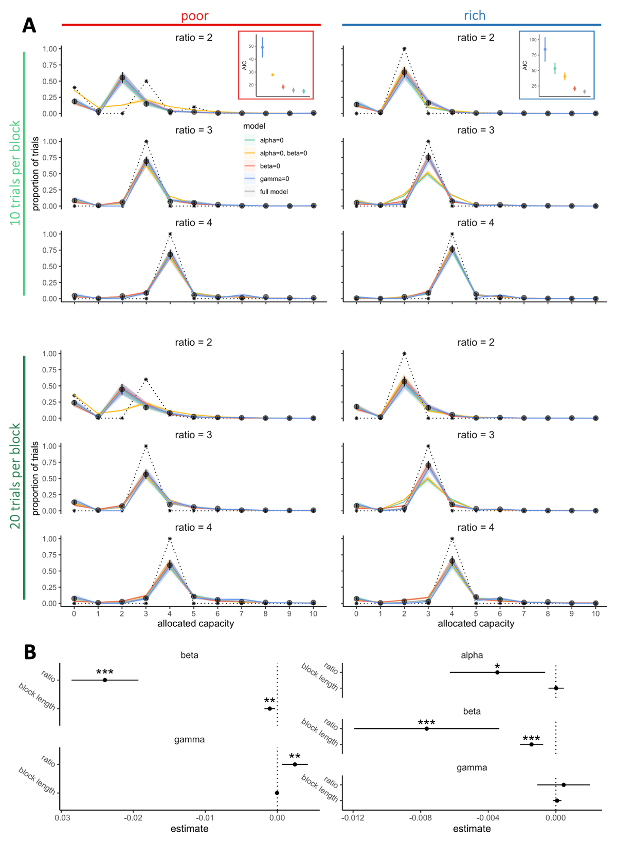
Figure 7
Participants sampling strategy considers exploration and individual risk aversion features. A. Probabilities to allocate a capacity C from 0 to 10 depending on the environment richness (poor: left panels, rich: right panels) and the block length (10 trials per block: upper panels, 20 trials per block: lower panels). Black points represent the averaged observed probabilities across participants and vertical bars the s.e.m. Colours lines represent the averaged fitted probabilities for each model and the shaded areas the s.e.m. across participants and dashed black lines represent the optimal probabilities for each condition (model maximising only the expected reward). In each environment, the averaged goodness of fits across participants (AIC – Akaike information criterion) were estimated by fitting the data within each block (regardless of block length) using the five different models. Vertical bars represent s.e.m. across participants. B. Factors (alpha, beta and gamma) extracted from the model predicting the data the best (‘alpha = 0’ in the poor environment and ‘full model’ in the rich environment) regressed with the capacity ratio and block lengths using LMEM. Estimates represents the extracted coefficients of regressions (bars represents 95% confidence intervals). ‘*’: p <. 05, ‘**’: p < .01, ‘***’: p < .001. N = 20 in each environment.

Figure 8
Participants have a tendency to homogeneously allocate capacity amongst the sampled alternatives, but it has little impact on the outcome. A. Number of samples allocated to each sampled alternative depending on the capacity allocated C in the rich environment. Upper panels: allocation of samples maximising the reward (optimal). Lower panels: most frequent allocations of samples observed across participants as a function of capacity. The allocations representing at least 50% of the trials are displayed and their likelihood is reported. B. Distribution of the differences between observed and optimal standard deviations of the distribution of samples among the selected alternatives in each environment (e.g. if C = 4 and 2 samples are allocated in a first alternative while the last 2 samples are each allocated in a second and third alternative, the standard deviation of this sample allocation would correspond to sd ({2, 1, 1}) ≈ 0.577). Note that more homogeneous distributions tend to lead to lower standard deviations. C. Distributions of the mean differences between observed and optimal outcomes in each environment. In the last two panels, dots represent participants and include all trials for which the optimal number of alternatives sampled doesn’t reflect a pure breadth strategy (Mopt < C– see Materials and methods for more details) and a capacity allocated up to 10. Below each distribution are presented results of one-sample Wilcoxon test (‘***’: p < 0.001 – B) and one-sample t-test (‘.’: p < 0.10 – C). N = 20, each data point averages 130 to 221 trials.