
Table 1
Hypotheses on the contribution of prior knowledge to WM organized by Experiment.
| HYPOTHESIS | ALTERNATIVE HYPOTHESIS | EXPERIMENT |
|---|---|---|
| Under which conditions does LTM contribute to performance in a WM task? | ||
| A) Obligatory LTM hypothesis: There is always a contribution of episodic LTM. | B) WM overload hypothesis: Once a person’s WM capacity is exceeded, performance is influenced by episodic LTM. | 3 and 4 |
| C) Decision ambiguity hypothesis: Benefits of prior knowledge are specific to conditions in which there is no ambiguity about decisions of using WM or LTM. | 2 | |
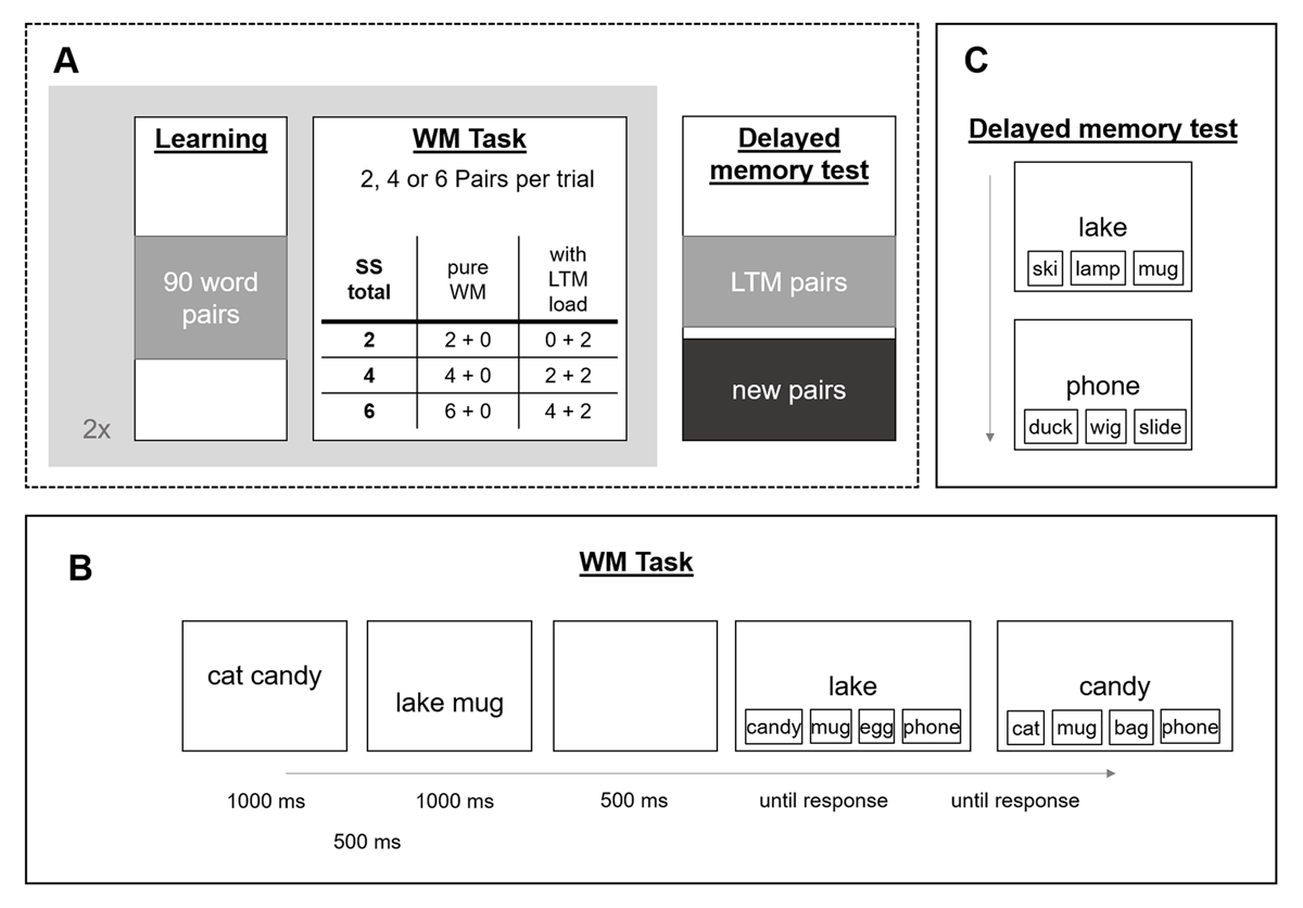
Figure 1
General procedure of Experiment 1 (A), with the WM task (B) and the Delayed memory test (C).
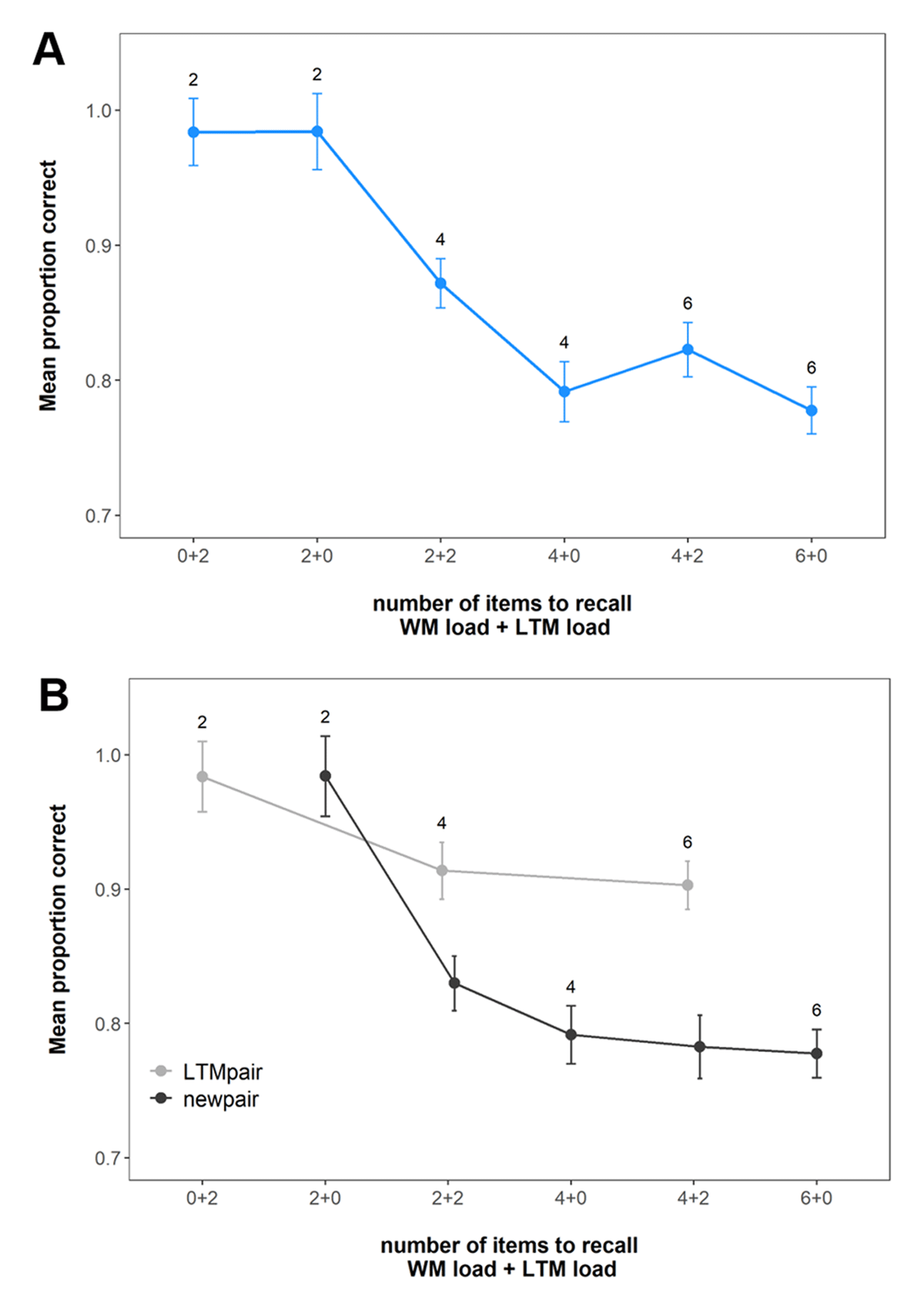
Figure 2
Mean immediate recall performance in Experiment 1. (A) shows the performance across all pairs at the set sizes. (B) shows the performance for the LTM and new pairs separately. The numbers in the figures show the total set size of the respective conditions. Error bars represent within-subject confidence intervals.
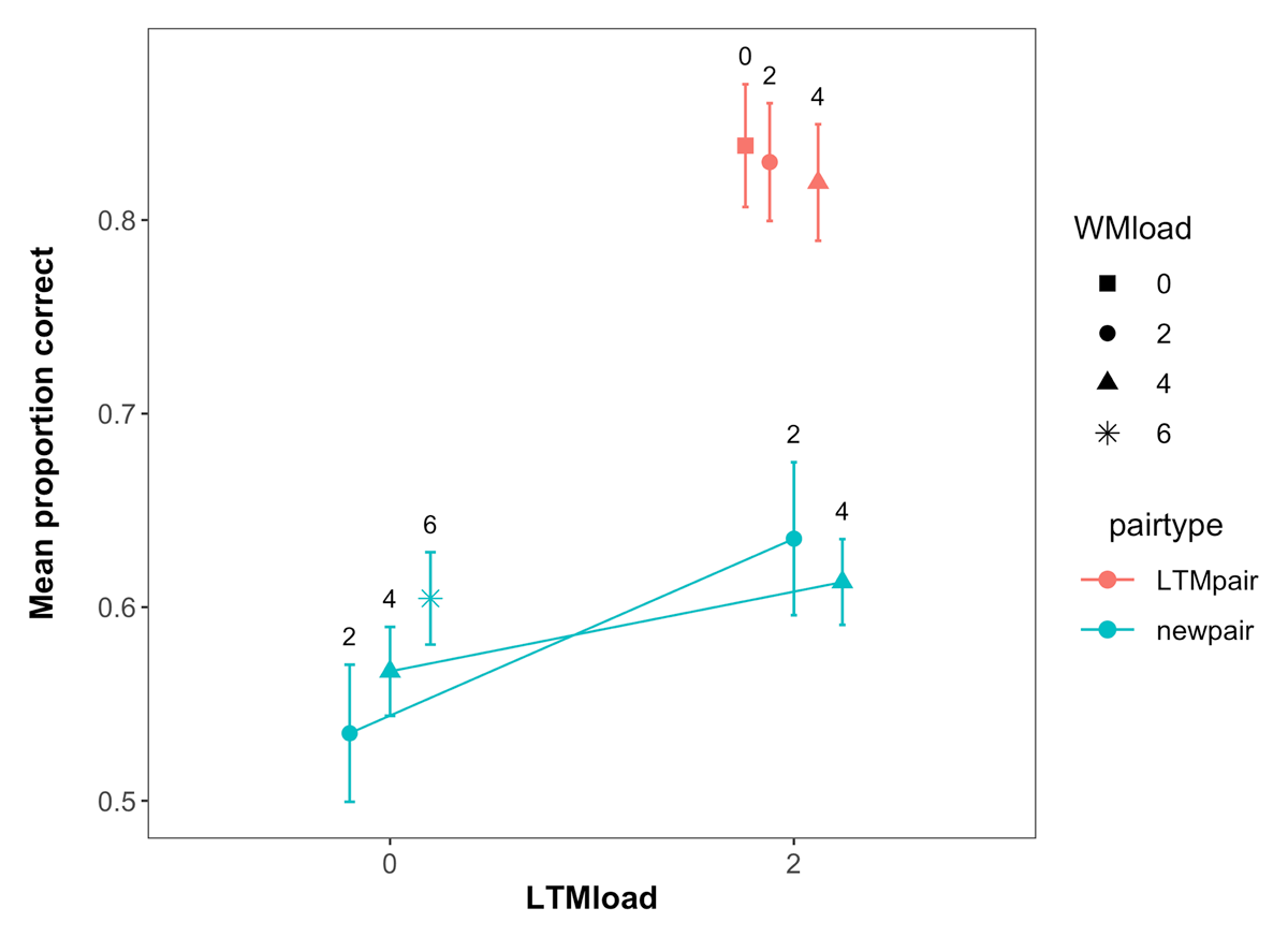
Figure 3
Mean performance in the LTM task across WM load, LTM load and pair type in Experiment 1. Labels represent the WM load. Error bars represent within-subject confidence intervals.
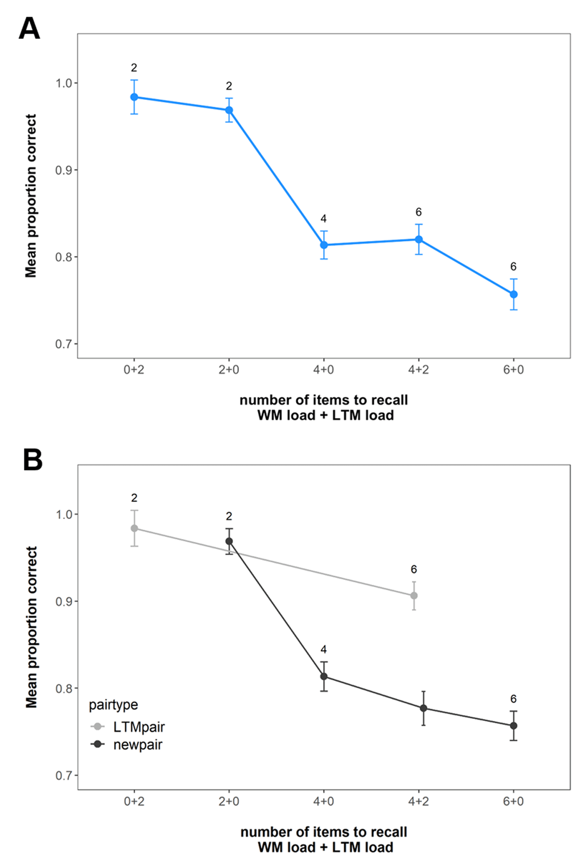
Figure 4
Mean immediate recall performance in Experiment 2. (A) shows the performance across all pairs at the set sizes. (B) shows the performance for the LTM and new pairs separately. Error bars represent within-subject confidence intervals.
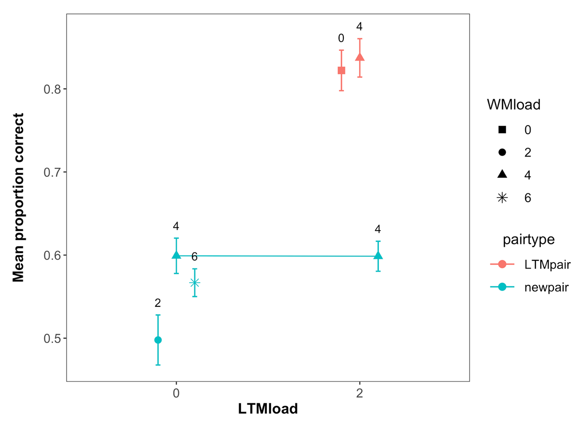
Figure 5
Mean performance in the LTM task across WM load, LTM load and pair type in Experiment 2. Labels represent the WM load. Error bars represent within-subject confidence intervals.
Table 2
The composition of trials at varying set sizes (SS) of Experiment 3 and 4.
| SS | NEW – NEW | OLD – NEW (MISMATCH) | OLD – OLD (MATCH) |
|---|---|---|---|
| 2 | x | x | |
| x | x | ||
| x | x | ||
| 3 | x | x | x |
| 4 | 2x | x | x |
| x | 2x | x | |
| x | x | 2x |
[i] Note: Rows represent the possible compositions at each of the set sizes. For instance, at set size 2, trials consisted of either (A) one new-new and one mismatch pair; (B) one mismatch pair and one match pair; or (C) one new-new and one match pair.
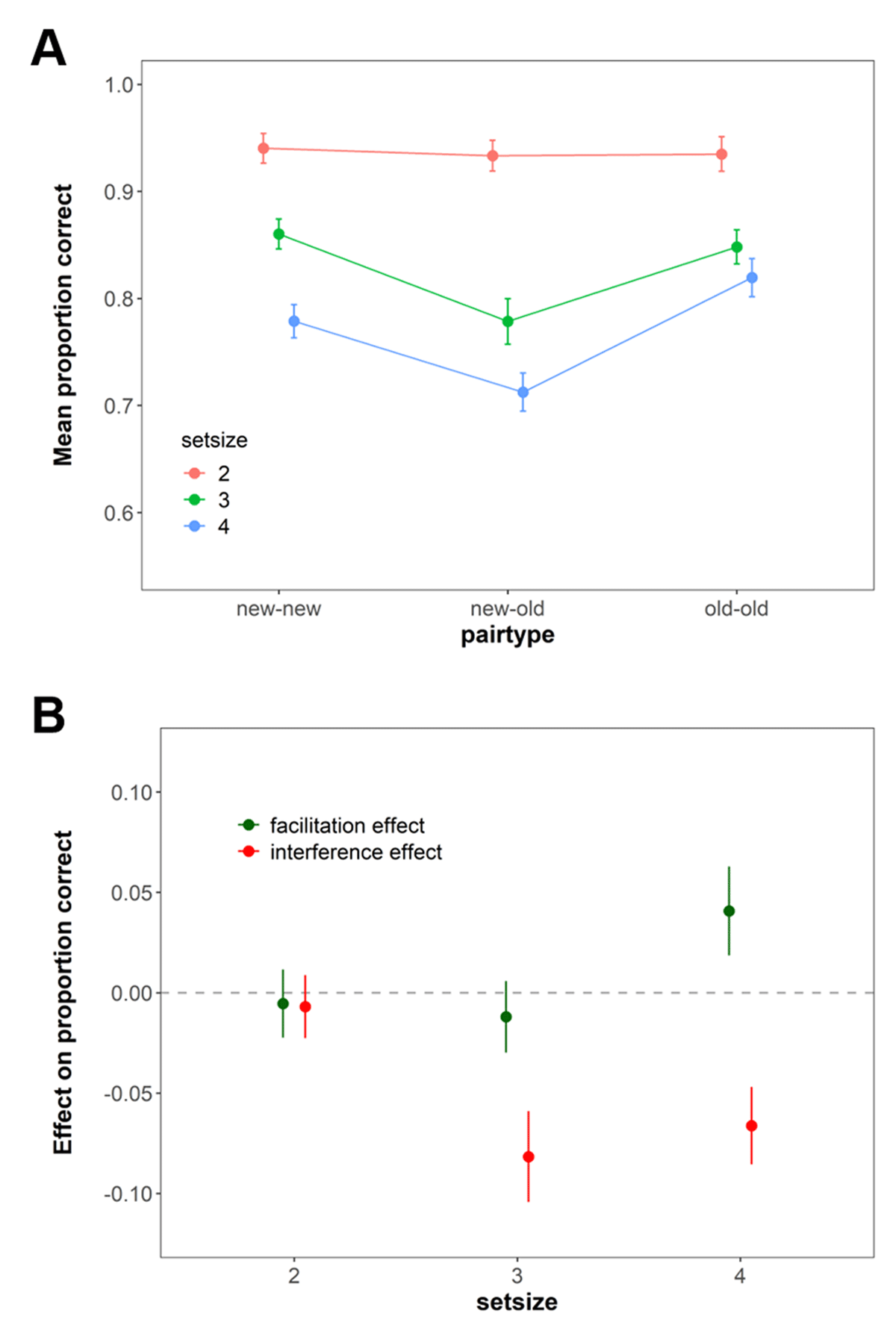
Figure 6
Mean immediate recall performance in Experiment 3. (A) shows the performance across all pairs at the set sizes. (B) shows the proactive facilitation (difference between old-old and new-new pairs) and interference effects (difference between. old-new and new-new pairs). Error bars represent within-subject confidence intervals.
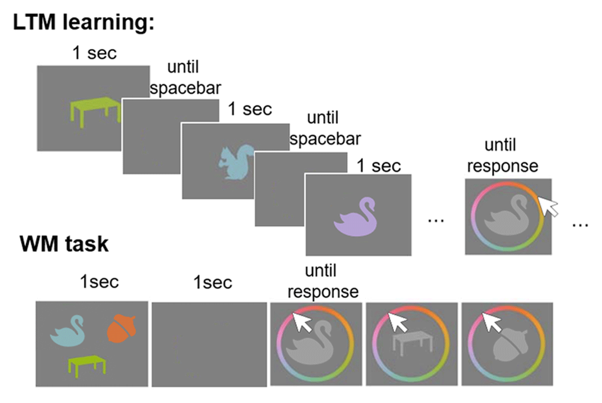
Figure 7
General procedure of Experiment 4 showing the LTM learning phase with the continuous reproduction test; and the flow of events in the WM test, here a set size 3 trial is depicted.
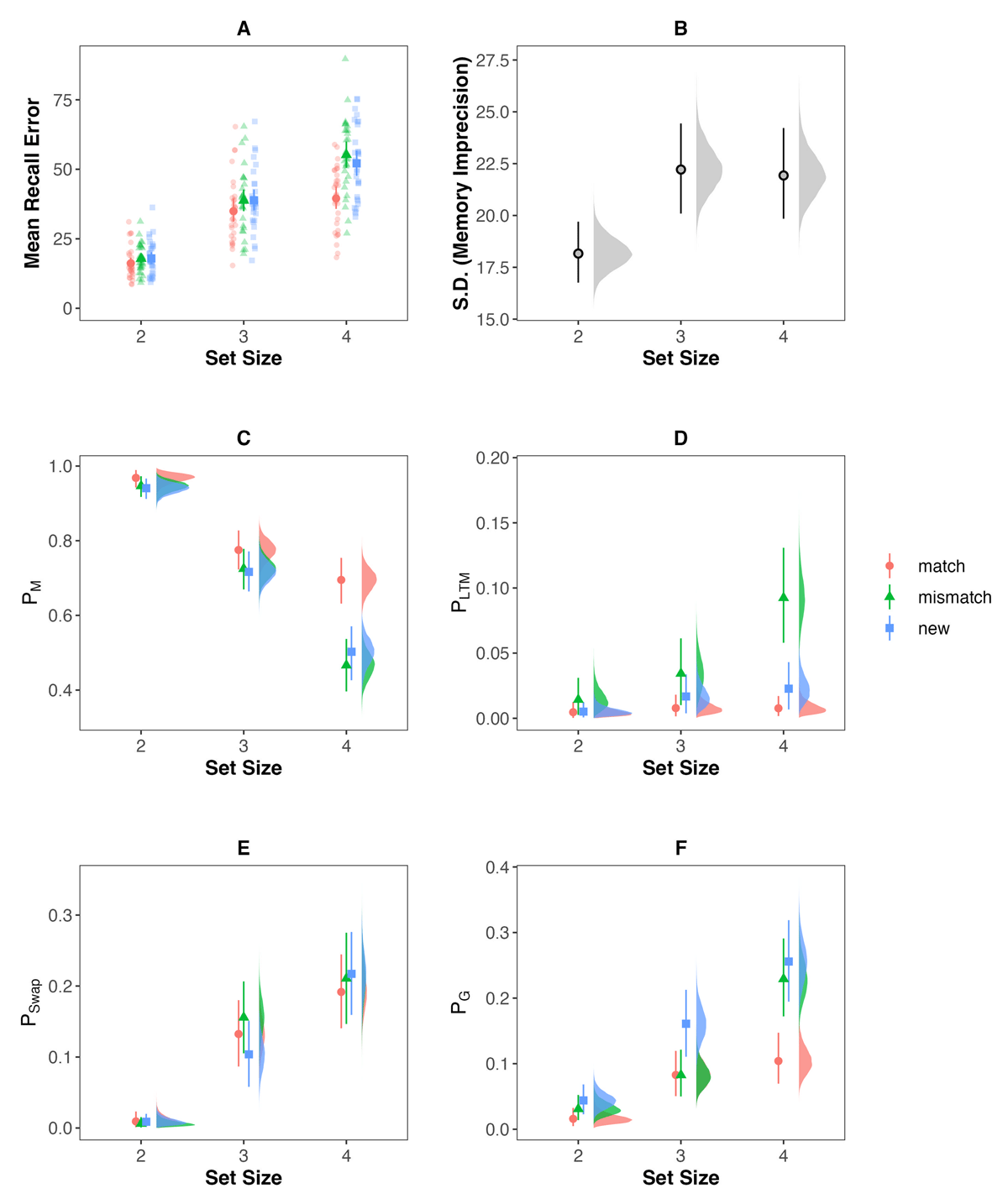
Figure 8
Descriptive plot of mean recall error (A) and estimated model parameters of the Bayesian hierarchical mixture modeling (B–F) of the behavioral performance in the immediate recall task of Experiment 4. The descriptive plot (A) illustrates the performance of all subjects (transparent points) as well as mean performance and the standard error. The plots of the model parameters show the full posterior distribution as well as the posteriors mean and 95% highest density interval.