
Figure 1
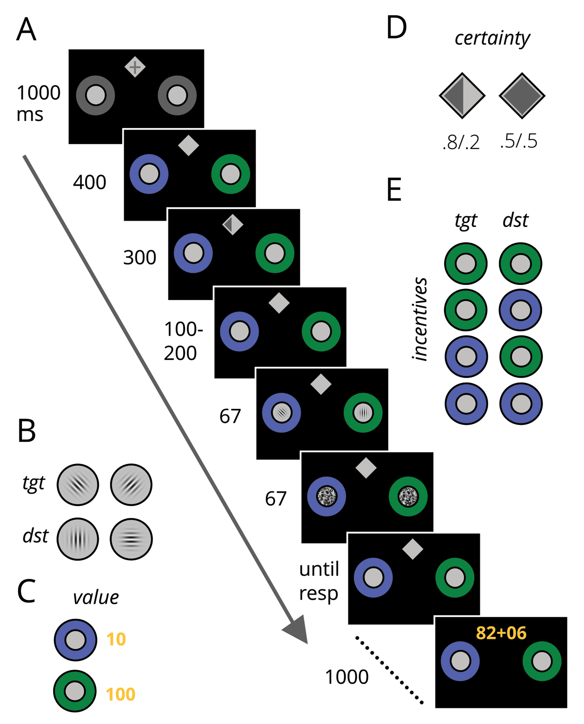
Experimental task. A) An example trial. Participants reported whether the target gabor was oriented clockwise or counterclockwise (B) the distractor was a gabor presented on the cardinal axis. C) Incentive value cues offered high (100) or low (10) point values. D) Spatial certainty cues were informative (p = .8) or non-informative (p = .5) regarding the upcoming target location. E) Incentive value cues were presented using 4 different configurations. tgt = target location, dst = distractor location, ms = milliseconds.
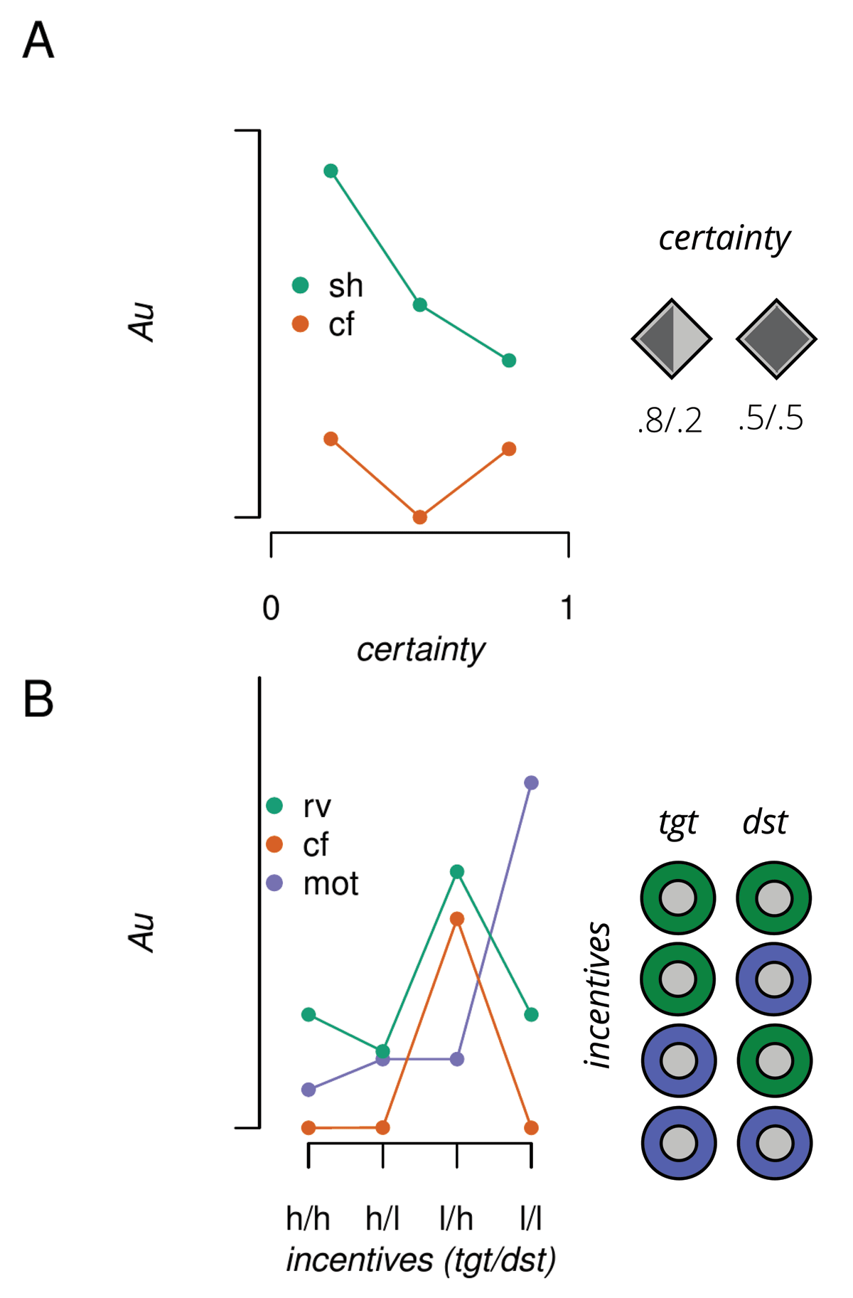
Figure 2
Theoretical predictions for the influence of spatial certainty and incentive value cues. A) Predicted RTs in arbitrary units (Au) given a selection-history (sh) or counterfactual (cf) encoding of the spatial cue. B) Same as A but for the influence of incentive value cues given relative value (rv), cf or motivational (mot) encoding. tgt = target location, dst = distractor location, h = high value, l = low value.
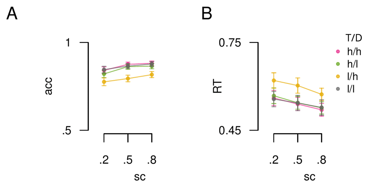
Figure 3
Influence of spatial certainty and incentive value. A) Group mean accuracy data plotted by spatial certainty (x-axis, sc) and incentive value condition (lines). B) RT data plotted in the same format as panel A. T = target location, D = distractor location, h = high value, l = low value. Error bars reflect standard error of the mean (SEM).
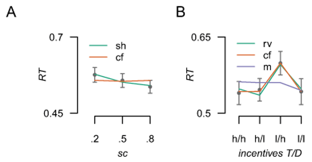
Figure 4
Model predictions plotted against the data for the influence of spatial certainty and incentive value. A) The influence of spatial certainty; the anticipatory (sh: selection history) and counterfactual (cf) model predictions plotted against the observed group average RT data (points). B) Predictions for the anticipatory (rv: relative value), counterfactual and motivational salience (m) models against the observed data. T = target location, D = distractor location, h = high value, l = low value. Error bars reflect standard error of the mean (SEM).
Table 1
Reliability of the key behavioural effects.
| EFFECT | R | DF | P |
|---|---|---|---|
| SC | 0.696 | 145 | 1.29e–22 |
| IVi | 0.926 | 145 | 2.40e–63 |
| IVii | 0.908 | 145 | 1.18e–56 |
| IViii | 0.828 | 145 | 3.48e–38 |
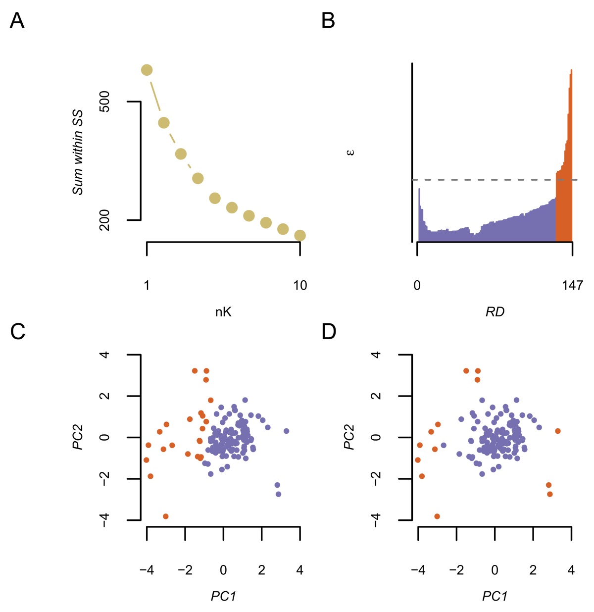
Figure 5
Sorting outcomes from application of k-means and OPTICS clustering algorithms. A) Sum of within sum of squares (SS) for each cluster solution (nK: x-axis) from the k-means algorithm. B) Data points ordered (x-axis) by Reachability epsilon distance (y-axis) by the OPTICS algorithm. C) The first two principal components of the feature space for the clustering analysis, where each participant is plotted as a point. Colour dentotes cluster group membership as found by the k-means algorithm. D) Same as C, except denoting group membership as found by the OPTICS algorithm. PC = principal component.
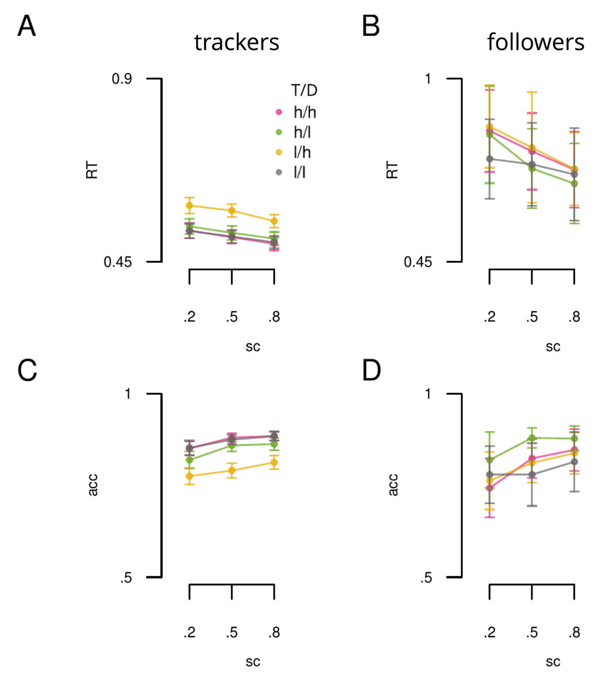
Figure 6
RT and accuracy data plotted separately for the 2 cluster groups. A) Showing RT data across spatial certainty (sc: x-axis) and incentive value (lines) for the trackers group (N = 131). B) Same as A, but for the followers group (N = 15). C) and D) Accuracy (acc) data plotted according to the same conventions as A and B. Error bars reflect SEM. T = target location, D = distractor location, h = high value, l = low value.
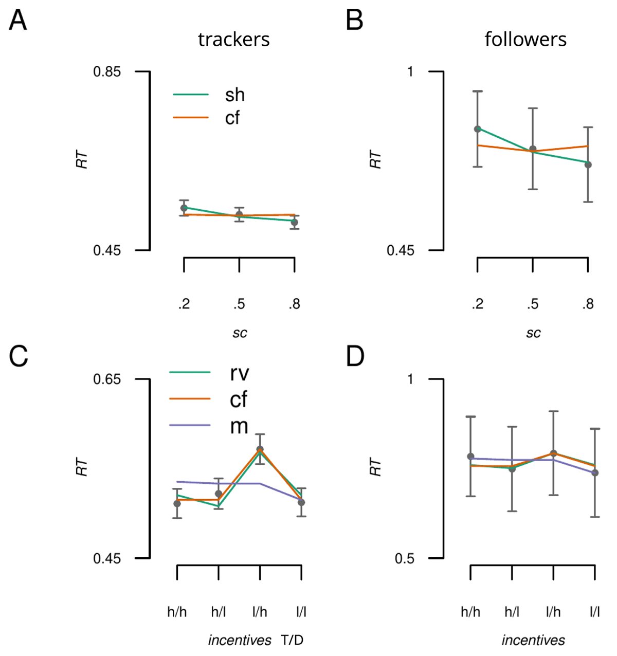
Figure 7
Model predictions plotted against the data for the trackers and followers groups. A) Response to spatial cues for the tracker group; anticipatory (sh: selection history) and counterfactual (cf) model predictions against the observed group average RT data (points). B) Same as A except for the followers group. C) Predictions for the anticipatory (rv: relative value), counterfactual and motivational salience (m) models against the observed influence of incentive values for the trackers group. D) Same as C but for the followers group. T = target location, D = distractor location, h = high value, l = low value. Error bars reflect standard error of the mean (SEM).