
1. Introduction
The Mediterranean basin, a highly fragmented seascape made up of smaller ‘micro-regions’ and semi-enclosed sub-basins, provided Mediterranean societies in the Late Bronze Age (LBA) (1450–1075 B.C.) a range of opportunities to interact, exchange goods and ideas, and manage risk through maritime movement (Horden & Purcell 2000). Arguably beginning with Braudel’s (1949; 1972) seminal work on the Mediterranean as a basin, more recent studies have continued to underscore the uniqueness of its complex geography for connectivity, interaction, and human mobility (Abulafia 2011; Broodbank 2013, 2016; Horden & Purcell 2000; Knapp, Russell & van Dommelen 2021; Malkin 2003; 2011; Renfrew 1972; Tartaron 2013). From this perspective, the Mediterranean can be viewed as a region with variably permeable boundaries that stretch inland, connecting and integrating beyond just its sea and coastline (Broodbank 2013; Knappett 2018; Leidwanger & Knappett 2018; Leidwanger et al. 2014).
Traditionally, interaction in the Late Bronze Age (LBA) Mediterranean has been explored archaeologically through a socio-economic, socio-cultural lens, with a focus on ceramic imports acting as proxies for long-distance contact (Cline 1994; Cline 1995; Cline 2009; Burns 2010; van Wijngaarten 2002; van Wijngaarten 2012), leading to broad reconstructions of maritime routes based on the patterns of suspected provenance and deposition (Papageorgiou 2008; Pulak 2009; Watrous 1992: 167–192, figs. 10–11). Although such approaches stressed the significance of seasonal winds, cabotage, and harbour hopping for reliable long-distance maritime mobility (Bass et al. 1967; Phelps, Lolos & Vichos 1999; Yon & Sauvage 2014), few have considered these factors in more formal modelling studies in the LBA Aegean and east Mediterranean.
The present paper considers the implications of seasonality and wind patterns for relative ease of maritime mobility between Crete and the east Mediterranean during the LBA. Building on earlier work (Alberti 2018; Arcenas 2021; Jarriel 2018; Jarriel 2021; Safadi 2019), it estimates sailing time and relative cost of travel, and reconsiders a previous distance-limiting null-model that only used Euclidean distance as an estimator for connectivity in the Mediterranean (Gheorghiade, Price & Rivers 2023; Gheorghiade 2020). These preliminary results are compared with ceramic imports from the site of Kommos, a key LBA harbour on the southern coast of Crete.
2. Modelling Mobility in the Bronze Age East Mediterranean
Early modelling of Aegean maritime spaces by Broodbank (2000) highlighted the importance of the maritime environment for early seafaring and interaction by Neolithic and Early Bronze Age (EBA) societies in the Cyclades. For the Middle Bronze Age (MBA), an ‘imperfect optimization’ model for maritime interaction also considered changes in the structural properties of the larger network under duress (Knappett, Evans & Rivers 2008; Knappett, Rivers & Evans 2011). Such approaches relied on Euclidean distance and sailing technology as significant considerations of ‘cost’ for accessibility and mobility across maritime spaces.
In recent years, formal models of maritime environments sought to create more dynamic representations of space that affected a range of human factors (i.e., experience, risk assessment) that impacted the performance and sailing time for a variety of vessels in the Mediterranean (Safadi & Sturt 2019). Distance travelled on such cost-surfaces was calculated using a range of variables such as wind, waves, speed, vessel capability, and seasonality from an origin point for both daily (Leidwanger 2013; Jarriel 2018) and hourly (Safadi & Sturt 2019) estimates. The use of detailed meteorological data with a range of software (various GIS, sailing simulation software) has also enabled the simulation of routes in the Mediterranean for the Greco-Roman period (Arcenas 2021; Gal, Saaroni & Cvikel 2021a), but also the EBA Cyclades (Jarriel 2018; Jarriel 2021), the Caribbean (Slayton 2018), and a historical map of the South China Sea (the Selden Map of China, see Perttola 2021). More recently, Fernandez and Aragon (2022) combined GIS and social network analysis (SNA) to model coastal navigation and cabotage in the early Iron Age west Mediterranean. Of these, the Stanford Geospatial Network Model of the Roman World (ORBIS) (Arcenas 2021) represents a pioneering digital resource that can be used to calculate the cost of connectivity (time and expense) across the vast Roman transportation network both over land and sea.
3. Archaeological Evidence
The focus of this study is the LBA eastern Mediterranean, and specifically mobility from the LBA site of Kommos on the south coast of Crete (Figure 1) and the east Mediterranean. Kommos sits on the coast overlooking the Libyan Sea, and with its specialised port facilities and identified ship sheds (Shaw & Blackman 2020), it is one of the few examples of purpose-built harbour facilities in the Bronze Age Mediterranean (see discussion in Mourtzas & Kolaiti 2020; Mourtzas & Kolaiti 2021). Ceramic evidence from Kommos points to the existence of a widespread network of trade with the wider Mediterranean, with imports identified from Kythera, the Cyclades, mainland Greece and further afield from Cyprus, Egypt, the Levant, Western Anatolia, and Sardinia in the west Mediterranean (Day et al. 2011: 552–4; Gheorghiade 2020; Rutter 2000; Rutter 2017; Tomlinson et al. 2010: 218). This makes Kommos one of the most diverse centres for imports on Crete and the Aegean, and a site where imports are present consistently throughout the LBA (Rutter 2017). Kommos was certainly not in isolation, nor was this distribution pattern unidirectional. Aegean-type ceramic exports have been found at a number of LBA sites along the east Mediterranean coast, highlighting the presence of extensive maritime-based interaction networks operating in the east-central part of the basin. The two other sites discussed here in conjunction with Kommos, Marsah Matruh (Hulin 2019) on the Egyptian coast and Maa-Palaeokastro (Georgiou 2012) in Cyprus (Figure 1), both have evidence of LBA Aegean-style ceramics, suggesting their participation in wider Aegean and Mediterranean networks of mobility and trade. These two sites were chosen for the present paper as spatially distinct points/nodes to give an indication of relative cost of travel across the eastern Mediterranean Sea; however, they should not necessarily be taken as the most important sites in the network.
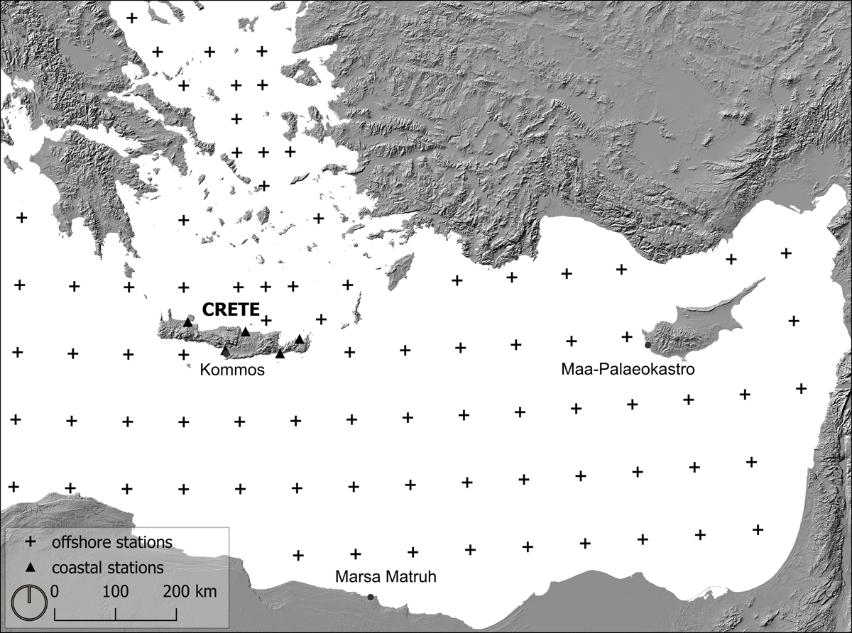
Figure 1
Location of wind data points. Map illustrates both offshore (+) and coastal (▴) data. The offshore data was extracted from the Med-Atlas database (Med-Atlas Group 2004), while the coastal data points were taken from the Hellenic Meteorological Service (currently available data from 2022). The extent of the map is the computational area used in the cost surface analyses. The three sites considered in this study are also illustrated: Kommos on Crete, Marsa Matruh on the northern coast of Egypt, and Maa-Palaeokastro on Cyprus.
Archaeologically identified shipwreck cargoes and ship anchors provide the best evidence for assessing LBA ship size and characteristics. The oldest surviving examples are the Uluburun and Cape Gelidonya shipwrecks off the south coast of Turkey (Bass et al. 1967; Bass 1991; Knapp 2018: 51; Pulak 1998; Wachsmann 1998), although a recently identified wreck on the south coast of Turkey, in the Kumluca district, might be an even older wreck dating to the 16th–15th century B.C. (Öniz 2019). A replica of an 18th Dynasty Egyptian vessel, named Min of the Desert, was created in 2008 based on reliefs from Hatshepsut’s Punt Exhibition at Deir el-Bahri and other archaeological evidence of ships from the sites of Wadi Gawasis and Ayn Sokhna (Couser & Vosmer 2009; Ward et al. 2012). Other ships are also known from iconography, but only a few ancient ships have been replicated for collecting sailing performance data (Johnston 1985; Simandiraki 2005; Van de Moortel 2017). Therefore, given the wide variability in performance results, we follow previous estimates (Leidwanger 2013) and rely on sailing performance data derived from sea trials undertaken by the Kyrenia II vessel, a replica of a Greek ship dating to approximately 300 B.C. that was excavated off the coast of Cyprus (Cariolou 1997; Katzev 1990; Katzev 2005). Although this ship dates nearly a millennium later, it is an acceptable point of reference for this preliminary analysis of open water voyaging. While the results are likely an overestimation maximum sailing performance of Bronze Age vessels, the data from the Kyrenia II provides a range of expected values for seasonal mobility and are used here to assess the relative accessibility between different regions. Furthermore, a more recently reconstructed replica of a 5th century B.C. ship discovered 70 metres off the coast of Kibbutz Ma’agan Mikhael (Palzur & Cvikel 2021) conducted short distance sea trials from Haifa to Jaffa and from Haifa to Cyprus with resulting data comparable to that of the Kyrenia II (Gal, Saaroni & Cvikel 2021b).
4. Euclidean Null Models
For the prehistoric Aegean, 100–150-kilometres have been the accepted upper threshold for a day’s sailing distance under favourable conditions (Broodbank 2000: 345; Knappett, Evans & Rivers 2008: 1014; see also Leidwanger 2013). Leidwanger (2013) notes that Greek and Roman sources posit a similar average between 100–125-kilometres for ideal maritime sailing. This distance threshold, when considered in Euclidean space, provides a misleading, albeit, useful first estimate of potential connectivity across maritime space. For example, an earlier distance limiting null-model (Gheorghiade 2020; Gheorghiade, Price & Rivers 2023; Bakker et al. 2021) considered the extent of potential connectivity between coastal sites on Crete and sites across the larger Mediterranean identified based on imports (Figure 2a, b). Here, Euclidean distance was a key element in connecting sites (or nodes), all of which were selected due to the presence of imports datable to the LBA. We used a simple attachment protocol, or connection parameters, where all sites (nodes) that were not further apart than a maximum geographical distance S, were linked. This maximum geographical distance ranged from 150 to 500-kilometres. We considered 150-kilometres, as the accepted upper threshold for a day’s sailing distance under favourable conditions, whilst 500-kilometres was the upper threshold at which all sites (nodes) connected in the network. This model ignored wind speed, direction, or currents, but highlighted changes in potential connectivity across the basin at various distance thresholds (Gheorghiade, Price & Rivers 2023).
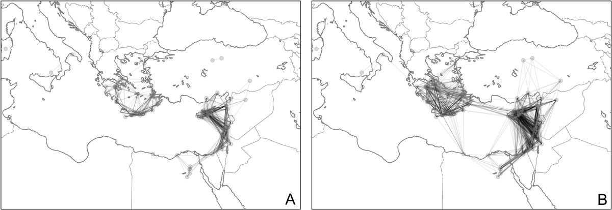
Figure 2
Distance-limiting null network models for the eastern Mediterranean based on Euclidean distance as a measure of potential connectivity. (a) represents the network with an inputted upper threshold of 200-kilometres; (b) represents the network when an inputted upped threshold of 450–500-kilometres is considered. (b) highlights the scale at which south Crete, and the site of Kommos, connect with the northern coast of Africa for the first time. After Gheorghiade, Price & Rivers (2023).
For example, Figure 2a highlights two distinct clusters at the 200-kilometre range: the Aegean centered on interaction among sites in Crete, the Cyclades, Dodecanese, mainland Greece and the west Anatolian coast, and another centered on Egypt and the Levantine coast. Interestingly, this is indeed what is seen in ceramic assemblages during the Middle Bronze Age (see also Knappett, Rivers & Evans 2011), where maritime contact with Crete is almost entirely limited to within the southern Aegean. Increasing this threshold to 450–500-kilometres (Figure 2b) highlights the scale at which Kommos connects to the northern coast of Africa acting as a bridging node for these smaller clusters or “small worlds” as defined by Tartaron (2013). As a heuristic exercise, this null model illustrates how Euclidean distance estimates alone provide a narrow and limited understanding of maritime spaces.
In the present study, we incorporate wind speed and direction variables in a cost surface analysis to explore how environmental conditions distort these distances, and to consider how seasonality affected maritime mobility in the east Mediterranean. We compare the relative accessibility of Kommos on Crete, to and from Marsah Matruh on the north coast of Egypt and Maa-Palaeokastro in Cyprus as two example points. Our aim is to build a more nuanced picture of potential maritime mobility that can be used for future exploration of maritime networks of interaction, mobility, and trade between Crete and the east Mediterranean during the LBA.
5. Wind Data and Parameters
Amongst a potentially wide array of variables that can be considered when modelling maritime movement, we prioritised surface wind data as it would have been one of the major factors determining the effectiveness of travel by sail in the LBA east Mediterranean. We did not consider the cost of maritime propulsion by oar in this study, which may have been more important for coastal travel. The Wind and Wave Atlas of the Mediterranean Sea Project (Med-Atlas) (Med-Atlas Group 2004) provides wind data in this analysis. The Med-Atlas collected wind and wave data from 935 stations across the Mediterranean over a 10-year period (1991–2002). It must be noted that while the use of modern data for modelling prehistoric phenomena is not without concerns, it is explicitly used here to produce heuristic models (rather than reconstructions of routes) of maritime movement. The goal is to explore how mobility can be expected to have been limited or favoured by certain conditions, and how these models might compare to patterning seen in archaeological assemblages. Nonetheless, as Murray (1987) has demonstrated, ancient winds in the Aegean and east Mediterranean can be considered roughly equivalent to present day metrics (see also Gal et al. 2021a). Moreover, the Med-Atlas project data employed here exclude measurements of more severe weather patterns as exacerbated by global warming over the last 20 years.
For the present modelling exercise, we included data for the summer and winter seasons, each comprised of three months: June, July, August and October, November, December, respectively. Although most seafaring in the Mediterranean would have most certainly occurred during the summer months (Bushnell 2016: 19–20), we included data from the winter seasons for comparison, to highlight the impact of seasonality and its constraints on potential maritime mobility. We employed the seasonal average of wind data as prevailing summer and winter winds are the strongest and most reliable for sailing. In addition, comparing winter and summer is a relatively straightforward method for considering seasonality in maritime models. As our study focuses on Crete, the wind data were collected from 82 separate offshore stations located within our study area (Figure 1, crosses), most of them buoys deployed at approximately 50-kilometre (1-degree) intervals (areas in the Sporades and North Aegean islands are approximately 25-kilometres apart or 0.5-degree intervals).
Modern wind data from five meteorological stations on the island (Figure 1, triangles), were also included. These data were acquired from the Hellenic National Meteorological Service (HNMS) website as monthly measurements. These were converted into direction in degrees and kilometres per hour to be aggregated into the dataset with Med-Atlas station data. This dataset slightly offsets the large gaps in coastal data, as the Med-Atlas only provides offshore data. Coastal wind data are significant in maritime modelling because wind patterns are largely influenced by landforms and can change both wind direction and speed significantly along the coast of landmasses. This is not an ideal dataset for prehistoric modelling, but it is readily accessible, fits the aim of this preliminary study and highlights the effect of landmasses on coastal and maritime travel. Although our focus here remains on long-distance travel for maritime models, the importance of coast hugging and island-hopping strategies (Gal, Saaroni & Cvikel 2021a) are considered more informally in the discussion.
6. Data Processing
The R computing environment was used to create a workflow (Spencer & Gheorghiade 2023) that extracted the data from the Med-Atlas frequency tables (Med-Atlas Group 2004) and converted them into values that could be interpolated and used in the cost analysis. A file was produced for the chosen subset of Med-Atlas data, which included, for each station, the latitude, longitude (coordinates for direct input into GIS), U and V components (common format of directional data for easy integration with other datasets), average speed (both in native m/s unit and converted into km/h), the average direction (in both degrees and radians), and the final corrected average wind direction in degrees (which is the final direction data that was used in analyses). The orientation data (wind direction) is a circular dataset (0–360 degrees), where 0 and 359 are both a northerly direction but when averaged would suggest a southerly direction. This requires straightforward trigonometric functions to produce averages of the observations at each station and generate a continuous data surface for analysis.
To transform the variables before they can be interpolated to produce a surface approximation, first the direction is converted into u and v components, representing east-west and north-south components respectively. Wind speed (ui) and wind direction in degrees (θi) are used in the following equations to produce the components which are weighted by their magnitude (or wind speed) (Grange 2014).
As these u and v components were calculated for every measurement extracted from the Med-Atlas database, the workflow also averaged all observations (for both seasons separately) and multiplied the value by –1 to negate the wind direction since by meteorological convention, wind is defined by the direction it is blowing from, rather than the direction it is heading to (Grange 2014). These components were used in the interpolation function, and transformed back into an average direction, () in degrees, with Eq. 3 by using the results from Eq. 1 and 2. If the resultant average wind direction () was <180 degrees, then +180 was required to produce the corrected average wind direction. This was straightforward in R with a condition in the script (Spencer & Gheorghiade 2023). To calculate average wind speed (Eq. 4), the u and v components were used and were converted from m/s into km/h.
To produce continuous surfaces for seasonal wind speed and direction that can be used to model the relative cost and time of travelling to and from Crete, a spline interpolation of the wind data was employed. Spatial interpolation aims to predict values of a variable based on the location in relation to known points (Nakoinz & Knitter 2016: 97-105). While there is no one best method of interpolation (Conolly 2020), spline interpolation methods are favoured for this study as they approximate data around known points, meaning the data value (speed or direction) at the precise location of a measurement station in the interpolated surface will be what was observed in the Med-Atlas dataset (see Hancock & Hutchinson 2006 for climate data example). Due to the regular distances between buoys in the Med-Atlas dataset, the resultant spline surface is a better approximation for the given study area (and was also used by Safadi 2016). As previously mentioned, with more coastal data, the maritime surface models can be greatly improved as coastal effects (particularly for the Aegean basin encircled by landmasses and dotted with islands) would be included in the interpolation surface. The present wind data was interpolated using a 1-arc second Digital Elevation Map (DEM) for the eastern Mediterranean available from the United States Geographical Service (USGS), which was clipped to our study area with a buffer of 15-kilometres to allow for edge effects in the interpolation. To speed up model computation considering the sparsity of available data points, the DEM was resampled to a 1000-metre resolution, since a smaller 30-metre resolution would be redundant and lead to potentially inaccurate interpolated surfaces (Conolly 2020: 126; Hengl 2006). Using the resampled DEM, four rasters were generated in R (Spencer & Gheorghiade 2023) for use in the cost surface analysis: separate wind direction and wind speed raster surfaces for both winter and summer seasonal datasets (Figure 3). These were then used to build the cost friction surfaces.
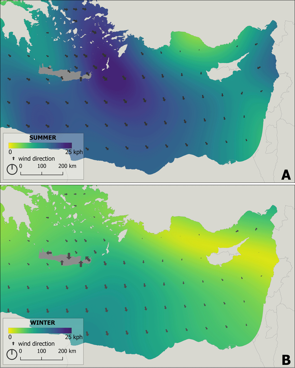
Figure 3
Wind speed (km/h) and direction (angle degrees) models for the summer (a) and winter (b). The continuous surface illustrates the interpolated average speed across the study area. The wind arrows are rotated in degrees to correspond to direction values, and their size corresponds to the average speed values observed at the measuring station. The locations of the arrows are the locations of the observation stations used in the dataset. The island of Crete is represented in dark grey. Note the relative difference in both strength and direction of wind from the Cretan coastal data compared to the offshore data, showing the effect of landmass on surface winds. Also note the relative decrease in wind speed along the Levantine coast in winter.
7. GIS and Maritime Cost Surface Building
To build the accumulated cost surfaces and construct travel times, we opted to make use of an earlier published ArcGIS Pro workflow (Alberti 2018). While not open source, the advantages of this are its ease of use and ease in adjusting a range of parameters as needed for analysis, as adding horizontal factors to cost surface analyses is not readily available in most GIS platforms. The deprecation of the ‘Path Distance’ tool in ArcGIS will require modification in future, however, for the present preliminary analysis, the outputs discussed below utilised the tool as is. An alternative to this workflow is the ‘gdistance’ package in the open-source R environment which can build accumulated cost surfaces from user-specified functions. The results can similarly be visualised in the form of time isochrones through simple raster calculations. Although we experimented with this ‘gdistance’ package, future work will explore this further.
Based on the interpolated wind speed and direction rasters, an accumulated cost surface was then generated. Frictional cost can be calculated in numerous ways (commonly used in archaeology as a function of movement over slope on land), but to calculate travel with a single square-sail ship on a maritime surface, a cost based on movement relative to wind direction was applied (more formally known as the ‘horizontal relative moving angle’). This required a table with calculated ‘horizontal factor’ values. For the present analysis, we employed and defined a table with the values 0.8, 1, or 3, following Leidwanger (2013). A reduced factor of 0.8 (meaning cost is reduced) relative to wind direction for 30°–79° was considered for helpful winds on a broad reach (i.e., behind the sailing craft). A factor of 1 for average, good wind conditions on a beam reach (i.e., right angle), at 0°–29° and 80°–120° implies a neutral position, and a factor of 3 for winds beyond the beam reach (i.e., heading upwind), beyond 120°, that is 121°–180° indicate relatively difficult conditions. As mentioned, these costs are based on data collected from sea trials of the Kyrenia II, resulting in sailing performance estimates in various conditions (Leidwanger 2013). In optimal wind conditions, a Mediterranean square-sail rig could travel an average speed of 4–6 knots per hour in open water, or approximately 7–11-kilometres an hour (Whitewright 2011; see also Leidwanger 2013). Since this data is derived from estimates based on Greek ships (i.e., 1st century B.C.), without comparable data for the LBA, we take these estimates as the upper bound of travel speed in ideal conditions. Thus, all results utilised a maximum value of 11.11-kilometres an hour, corresponding to 6 knots, as the estimated upper threshold. It is important to note that square-sailed ships could not sail into the wind, and any straight-line sailing (as presented in this paper) would have had to be done as part of one leg of a voyage (Forsyth 2022: 161) until winds changed direction. Despite this, single square-sail ships continued to be made and used into Late Antiquity, suggesting that “windward sailing ability was not that important in many cases” (Forsyth 2022: 161; Whitewright 2018: 40; Gal, Saaroni & Cvikel 2021b; Gal, Saaroni & Cvikel 2023). For return journeys that required sailing into the wind, multi-stop tramping would have undoubtedly been the norm (Forsyth 2022). Nonetheless, as for the aim of the present paper is to highlight the unpredictability of winter conditions for increased cost and the relatively small window of the optimal sailing season, we retain the values discussed by Leidwanger (2013).
As movement is directionally dependent, anisotropic accumulated cost surfaces were generated for each site (see Alberti 2018: 512 for cost functions used in the TRANSIT tool). These, in turn, were used to generate raster surfaces which measured distance by travel time. A comparison of these cost and travel time surfaces made it possible to determine relative mobility within our larger study area of the east Mediterranean. Figures 4, 6 and Tables 1, 2 present these results, illustrating the resulting seasonal sailing conditions for Kommos (Figures 4a, b), Marsa Matruh (Figures 5a, b) and Maa-Palaeokastro (Figures 6a, b).
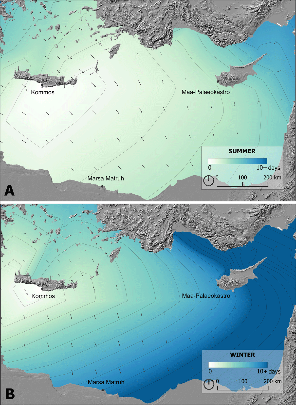
Figure 4
Cost in days with travel from Kommos on Crete, for summer (a) and winter (b). The number of days is illustrated from 0 (white) to 10+ (dark blue). Daily isochrones also show the limits of travel within the number of days. The prevailing wind speed and direction are illustrated by the arrow size and direction respectively, as in Figure 3.
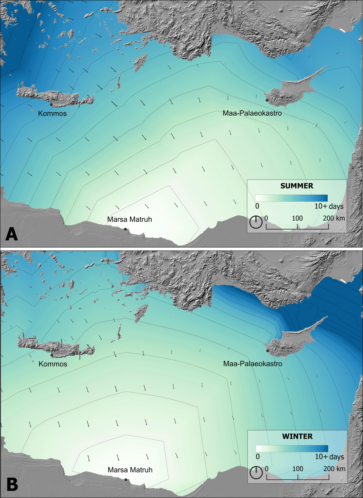
Figure 5
Cost in days with travel from Marsa Matruh on the Egyptian coast, for summer (a) and winter (b). The number of days is illustrated from 0 (white) to 10+ (dark blue). Daily isochrones also show the limits of travel within the number of days. The prevailing wind speed and direction are illustrated by the arrow size and direction respectively, as in Figures 3 and 4.
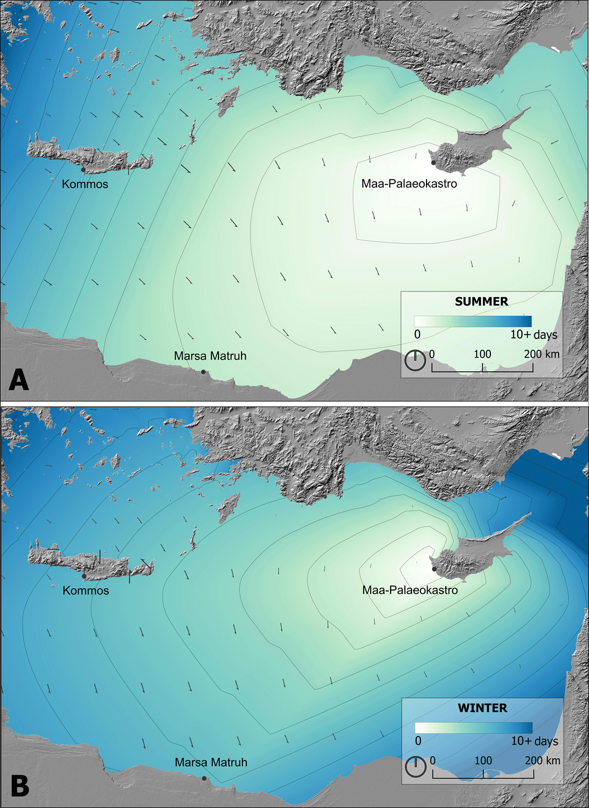
Figure 6
Cost in days with travel from Maa-Palaeokastro on south coast of Cyprus, for summer (a) and winter (b). The number of days is illustrated from 0 (white) to 10+ (dark blue). Daily isochrones also show the limits of travel within the number of days. The prevailing wind speed and direction are illustrated by the arrow size and direction respectively, as in Figures 3, 5.
8. Results
It is important to note that while coastal wind data would undoubtedly alter navigation (along with many other factors such as local sailing knowledge, coastal navigation practices, intra- and inter-regional contacts, provisioning needs), the aim of these models is not to reconstruct LBA sailing times. It is certain that considerations of cargo weight, crew size, and additional provisions would have affected speed and distance travelled. Moreover, even these ideal travel speeds implicitly assume that the speed remained constant throughout the voyage, unlikely to have matched the reality of maritime voyaging (Arcenas 2021). By taking seasonal averages, the present model also ignores the reality of daily changing weather conditions that could have prevented sailing journeys to be completed under ideal conditions (Arcenas 2021; Gal, Saaroni & Cvikel 2021a; Gal, Saaroni & Cvikel 2023), requiring stops that would have increased total travel time. For the present paper, therefore, we take a simple and coarse-grained approach, with the goal of assessing relative travel time and general navigability, under what could be considered ideal conditions. Consequently, we consider the models as indicators of the relative ease, in terms of sailing time and seasonal conditions, of maritime mobility between our selected sites (or nodes) to reassess previous prehistoric models based only on Euclidean distance.
8.1 Summer Season
The accumulated cost model shows that for the summer season, with the prevailing winds blowing south, sailing from Kommos towards the northern coast of Egypt would have been a relatively favourable journey (Figure 4a). Travelling at a maximum speed of 6 knots (Table 1), a ship could reach the coast on the second day, and the site of Marsa Matruh after two and half days (excluding coastal effects). The coast of Cyprus, and the site of Maa-Palaeokastro would be within reach in a little over three days.
Table 1
Cost of travel, measured in days of sailing (based on maximum speed of 6 knots) to the sites listed on the left based on the point of origin.
| FROM KOMMOS | FROM MARSA MATRUH | FROM MAA-PALAEOKASTRO | ||||
|---|---|---|---|---|---|---|
| SUMMER | WINTER | SUMMER | WINTER | SUMMER | WINTER | |
| Kommos | – | – | 7.19 | 3.67 | 6.41 | 6.37 |
| Marsa Matruh | 2.32 | 8.99 | – | – | 2.88 | 6.12 |
| Maa-Palaeokastro | 3.13 | 8.18 | 4.49 | 4.93 | – | – |
Sailing into the wind from Marsa Matruh towards Kommos in the summer (Figure 5a) would have been costlier, with a ship making the trip to Kommos in a week. Sailing towards Cyprus from Egypt, however, would have taken only four and half days, although presumably coast-hugging along the Levantine coast would have been preferred in this instance (Safadi & Sturt 2019).
By contrast, from Maa-Palaeokastro (Figure 6a), a ship sailing towards Marsa Matruh could reach its destination fairly quickly, towards the end of the second day. Reaching the eastern most point of Crete would take four and a half days, and Kommos six and a half days (disregarding possible coastal effects). With prevailing winds blowing against the direction of travel, sailing north from both Marsa Matruh and Cyprus would have been less than ideal during the summer months.
8.2 Winter Season
Despite the risks of winter sailing (Reger, 1994), for this exercise, we aimed to emphasise the impact of wind on the seascape compared to the preferable summer months. For the winter season, with speeds decreasing compared to the summer months, a ship sailing from Kommos (Figure 4b) towards the site of Marsa Matruh, would reach its destination at the end of the eighth day. Maa-Palaeokastro would also be within reach only after eight days, highlighting the impact of seasonal wind speed and direction on sailing potential compared to summer averages (Tables 1, 2).
By contrast, sailing north from Marsa Matruh (Figure 5b), first towards Crete, one would reach Kommos fairly quickly, in around three and half days, theoretically halving the travel time if the unpredictability of conditions were disregarded. To Maa-Palaeokastro from the north coast of Africa, an open water journey would take under five days, with little change from summer averages (Tables 1, 2).
Lastly, winter sailing from the coast of Cyprus at Maa-Palaeokastro (Figure 6b) is roughly the same towards both Kommos and Marsa Matruh, both resulting in a journey lasting a little over six days. Sailing into the wind from Marsa Matruh and Maa-Palaeokastro poses the biggest challenge in the winter for these models, whether at 6 knots (Table 1) or at a reduced maximum speed of 3 knots (Table 2). Concurrently, sailing times from every site are almost always affected in the winter months by a lower seasonal wind speed across the study area (Figure 3), which would make sailing in favourable directions slower.
Table 2
Cost of travel, measured in days of sailing (based on maximum speed of 3 knots), to the sites listed on the left from the point of origin.
| FROM KOMMOS | FROM MARSA MATRUH | FROM MAA-PALAEOKASTRO | ||||
|---|---|---|---|---|---|---|
| SUMMER | WINTER | SUMMER | WINTER | SUMMER | WINTER | |
| Kommos | – | – | 13.93 | 6.42 | 12.43 | 9.94 |
| Marsa Matruh | 4.48 | 15.75 | – | – | 5.52 | 9.86 |
| Maa-Palaeokastro | 6 | 13.16 | 8.54 | 7.96 | – | – |
9. Discussion
There are several implications from this modelling exercise, especially in comparison with the earlier distance limiting null-model (Gheorghiade, Price & Rivers, 2023; Gheorghiade 2020). Both models highlight the importance of Kommos as a south Cretan coastal node for maritime mobility in the eastern Mediterranean. An approximate distance of 466-kilometres, in the Euclidean distance model, Kommos only connected beyond its main Aegean “small world” cluster to Marsa Matruh, once the distance threshold was increased to 500-kilometres. However, the summer cost models here highlight the relative ease with which a ship sailing with prevailing winds travelling at 6 knots (although maximum performance was likely to have been closer to 3 knots) would reach the northern coast of Africa, that is within two sailing days. Equally, directionality is shown to be an important consideration disregarded in Euclidean distance models, as sailing north from Marsa Matruh was less costly in the winter, with an average sailing time of three and a half days. Nonetheless, as sailing in the winter months was more dangerous and difficult, these comparisons aim at highlighting the variability in cost (in time) when travelling during the summer and winter months due to prevailing wind directions with a square-rig ship.
Connecting to the Cypriote coast was likewise only possible in the null model through intermediary nodes, as the distance between these points is approximately 850-kilometres. However, our modelling has shown that with favourable winds in the summer, direct sailing from Kommos to Maa-Palaeokastro is estimated at just three days, covering a distance that is almost double that of travel to Marsa Matruh. Despite this optimistic estimate, it is likely that mercantile ships would have preferred coastal navigation to open water journeys, both due to the potential security afforded by quickly changing wind patterns, and access to a range of ports for goods and services. Nonetheless, this heuristic exercise highlights how changing seasonal winds and directionality impact sailing cost across open water, constraining when mobility between regions occurred, and the potential connectivity between ostensibly distant sites in the wider east Mediterranean.
Archaeological evidence of what might have travelled from Kommos across the wider Mediterranean is difficult to identify and remains frustratingly elusive. For example, during the LBA, specifically LM IIIA2–LM IIIB, workshops at Kommos started producing a new type of amphora, called the short-necked amphora in very large quantities (Rutter 2000). These the short-necked amphora are very standardised in shape, size, and production technique, suggestive of mass production (Rutter 2000: 5). Despite their popularity at Kommos, suggesting that they were likely produced and shipped out with their contents, they remain barely attested beyond the region surrounding Kommos (Day et al. 2011: 517). The analysis of 17 transport stirrup jars found in the Levantine port of Tell Abu-Hawam suggests a possible south-central Cretan origin (Ben-Shlomo, Nodaru & Rutter 2011). This tentative identification highlights a possible reciprocal exchange relationship between the southern coast of Crete—potentially via Kommos—and sites along the southern Levantine coast, or at the very least, the participation of these two regions in a wider zone of interaction within the east Mediterranean.
Despite lack of evidence for the spread of the short-necked amphora across the east Mediterranean in the LM IIIA2–LM IIIB period, it is in this period that imports at Kommos (Figure 7), are among the most diverse. They have been identified to have come from not only a wide range of sites across Crete itself, but also mainland Greece, Western Anatolia, the Levant, Cyprus, the Cyclades, Egypt and even Sardinia and mainland Italy. Imports from Cyprus are among the most common at Kommos, and although their association with a specific workshop or origin remains unknown, it can be reasonably suggested that interaction between these two regions was not an uncommon occurrence in the LBA. Whether these connections were direct, or the result of cabotage, remains up for debate (Knapp, Russell & van Dommelen 2021 for discussion). However, the presence of Sardinian, Italian, and Cypriote ceramics at Kommos, and of Cypriot ingots in Sardinia (Knapp, Russell & van Dommelen 2021), potentially suggests Kommos as an important stopping point within larger eastern and western Mediterranean maritime networks of mobility and exchange. Based on the present modelling, sailing from the Cypriot coast to Kommos would have resulted in a little over six days of travel, in both the summer and winter, in stark contrast to the distance only model, dramatically shrinking the distance for connectivity across the eastern basin.
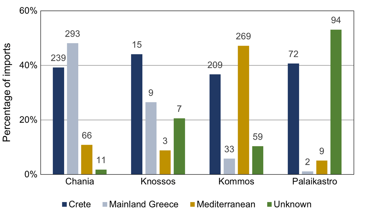
Figure 7
Comparison of percentages of ceramic imports and their provenance from four major LBA sites on Crete. The values on the bar labels represent quantities identified as imports. At Kommos, there are 209 identified imports from other Cretan sites, 33 from mainland Greece, 269 from the wider Mediterranean and 59 imports of unknown origin. Note that Kommos exceeds in both percentage (nearly 50% of imports are from the wider Mediterranean) and absolute quantities. Data from Gheorghiade (2020).
With an approximate distance of 740-kilometres, the sites of Marsa Matruh and Maa-Palaeokastro likely connected in the network model though intermediary nodes. Nonetheless, the wind modelling here shows that even in prevailing winter winds, sailing across open water with a maximum speed of 6 knots, would take six days, although ideal summer sailing conditions halved travel time between Egypt and Cyprus. We contend, however, that these estimates assume ideal travel conditions (i.e., consistent, favourable weather), without potential coastal or island stop-overs that would have extended the duration of the voyage. For merchant ships, this might indeed have been a more favourable strategy, both for risk reduction and off-loading and re-loading of cargo.
Given the likely overestimation of the performance characteristics of LBA sailing vessels, we also tested a maximum speed of 3 knots, or 5.56-kilometres an hour for each site (Table 2). The results, unsurprisingly, nearly doubled the sailing costs for both seasons. We might expect that for a LBA vessel, a more reasonable estimate of travel between Egypt and Cyprus might lie somewhere in between six to twelve days in the winter, and four to eight days in the summer. This estimate could be adjusted by considering additional factors such as weather changes that would prolong a journey, or other unexpected delays in ports of call that would impact total travel time.
Nonetheless, these results highlight how heuristic models incorporating seasonality and considerations of cost, measured in days of travel, can build on distance-limiting null models in exploring networks of connectivity across the east Mediterranean. Consequently, when we consider potential mobility or zones of interaction between sites in the Mediterranean, a measure of temporality can significantly alter networks defined only using Euclidean distance, forcing us to adjust the way we view zones of interaction by including both directionality and temporality.
9. Conclusion
This paper presented a preliminary exploration of maritime mobility through the application of wind data for exploring the seasonally variable costs of travel from Kommos on Crete to several indicative sites in the eastern Mediterranean. It highlighted the limitations of Euclidean distance only network models by emphasizing the difference in travel time when seasonality and wind direction were taken into consideration. As a heuristic model, it provided a baseline comparison for thinking about prehistoric maritime connections by highlighting how differences in seasonality increase the costs of travel across seascapes.
Nonetheless, this preliminary analysis can benefit from considerable adjustments. Other wind datasets with denser data points (e.g., Hersbach et al. 2023) would improve precision and accuracy of interpolated surfaces. More importantly however, the inclusion of coastal wind data for all landmasses would greatly nuance the results, specifically around landmasses, providing more accurate projections for both open water and coastal navigation, particularly in the island-laden Aegean Sea. For Crete, this is especially crucial as in many instances, the circumnavigation of the island was preferred to more difficult cross-mountain crossings (Chalikias 2009; Gheorghiade 2020). The effect of wind patterns on the coast also impacted the location and establishment of safe harbours (see also Safadi 2016). The friction costs assigned to travel with or against the wind could also be experimented with, to explore how sensitive the resultant travel times are to variable change (e.g., if beyond beam reach (>120°) is being penalised enough in Leidwanger 2013 for a LBA vessel). Other analyses such as least-cost-path (LCP) modelling (see Perttola 2021; Slayton 2018 for examples in maritime environments) could explore if there are certain areas or routes favoured by the environmental conditions modelled. LCPs could be used to reassess proposed maritime routes, for example like those of the Uluburun shipwreck (Pulak 2009). This ship has widely been suggested to have been travelling counterclockwise from its potential home harbour of Tell Abu Hawam, in a circuitous route stopping along the way at ports such as Tell el-‘Ajjul, Tyre, Sidon, Byblos, Crete and mainland Greece (see Pulak 2009: 298, Figure 97).
Acknowledging the complexity of maritime spaces and aiming for the development of better techniques for modelling mobility and interaction can contribute to testing long-held hypotheses on LBA trade routes, and the impact these connections might have had on the emergence and prominence of sea-facing communities. The site of Kommos, despite its significance as a harbour (Shaw & Shaw 2006), was also a ‘gateway community’ (Cline 1994: 87) for long distance goods. It was significantly positioned within Crete, connecting the large agricultural plain of its hinterland (largest on the island) with larger settlement clusters strung along the north coast (Gheorghiade 2020). Intra-island interaction is evident from the presence of open and closed vessel imports from Chania in the west, the Ierapetra isthmus in the southeast, and Palaikastro in the east (Gheorghiade 2020). Consequently, it becomes important to ask how maritime mobility and terrestrial centrality both contributed to the emergence and stability of coastal sites, such as Kommos, and how the growth of these sites influenced intra-island networks and hinterland communities. This question becomes especially crucial for understanding continuity, resilience, and reconfiguration of local and long-distance networks of interaction in the aftermath of pan-Mediterranean destructions that mark the end of the LBA. For example, how did these earlier maritime networks lay a foundation for later Phoenician mobility? The integration of environmental variables for modelling mobility can provide a more nuanced perspective on diachronic network change across maritime space.
Acknowledgements
We would like to thank Todd Whitelaw and two anonymous reviewers for their immensely helpful feedback and suggestions that greatly improved the content of the final draft. Thank you also to the organisers of the 2023 CAA session A Bridge too Far: Historical, Archaeological and Criminal Network Research, Marta Lorenzon, Arianna Traviglia, Lena Tambs, and Michela De Bernardin, for an inspiring session and for including our paper in the current volume. We also extend our gratitude to Justin Leidwanger for his help in facilitating access to the Med-Atlas dataset, without which the present analysis would not have been possible. Thanks are also due to the Centre of Excellence in Ancient Near Eastern Empires (ANEE, decision no. 352748). Open access funded by Helsinki University Library.
Reproducibility
The R script used for interpolating our data as well as a toy model are included for reproducibility at the following link: https://github.com/cspencer905/MedAtlasModelling. For the ArcGIS toolbox see Alberti (2018) below. The Wind and Wave Atlas of the Mediterranean Sea (Med-Atlas) data is available in electronic format provided by the Med-Atlas Group (2004) and cited below.
Competing Interests
The authors have no competing interests to declare.