

Figure 1
Justin Bieber. Note: This file is licensed under the Creative Commons Attribution-Share Alike 3.0 Unported license (https://commons.wikimedia.org/wiki/File:The_Bet_Justin_Bieber_y_T%C3%BA_Novela_Escrita_por_@Pretty_Jezzy_01.jpg).
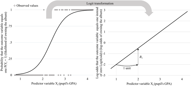
Figure 2
The logistic function describes the s-shaped relationship between a predictor variable Xi and the probability that an outcome variable equals one P(Yi = 1) (left panel, corresponding to Eq. 2); using the logit transformation, one can “linearize” this relationship and predict the log-odds that the outcome variable equals one instead of zero Logit(P(odds)) (right panel, corresponding to Eq. 3). Notes: Data are fictitious and do not correspond to the provided dataset.
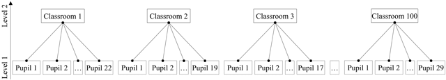
Figure 3
Example of a hierarchical data structure, in which N participants (pupils, lower-level units) are nested in K clusters (classrooms, higher-level units). Notes: Multilevel modeling is flexible enough to deal with this kind of unbalanced data, that is, having unequal numbers of participants within clusters.
Table 1
Summary of main notation and definition (level-1 and level-2 sample size and variables, as well as fixed and random intercept and slope).
| Sample size | N Level-1 sample size (number of observations) | K Level-2 sample size (number of clusters) |
| Variables | x1ij, x2ij, …, xNij Level-1 variables (observation-related characteristics) | X1j, X2j, …, XKj Level-2 variables (cluster-related characteristics) |
| Intercept | B00 Fixed intercept (average log-odds that the outcome variable equals one instead of zero Logit(P(odds)), when all predictor variables are set to zero) | u0j Level-2 residual (deviation of the cluster-specific log-odds that the outcome variable equals one instead of zero from the fixed intercept; the variance component var(u0j) is the random intercept variance) |
| Level-1 effect | B10, B20, …, BN0, Fixed slope (average effect of a level-1 variable in the overall sample; it becomes the odds ratio when raised to the exponent exp(B) = OR) | u1j, u2j, …, uNj Residual term associated with the level-1 predictor x1ij, x2ij, …, xNij (deviation of the cluster-specific the effect of the level-1 variable from the fixed intercept; the variance component var(u1j) is the random slope variance) |
| Level-2 effect | B01, B02, …, B0K, Necessarily fixed slope (average effect of a level-2 variable in the overall sample; it becomes the odds ratio when raised to the exponent exp(B) = OR) |
[i] Notes: For the sake of simplicity, no distinction is made between sample and population parameters and only Latin letters are used.
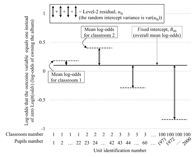
Figure 4
Graphical representation of the fixed intercept B00 and the level-2 residual u0j (cf. Eq. 4); the fixed intercept B00 corresponds to the overall mean log-odds of owning Justin’s album across classrooms; the random intercept variance var(u0j) corresponds to the variance of the deviation of the classroom-specific mean log-odds from the overall mean log-odds (here represented by the double-headed arrow for the 1st, 2nd, 3rd, and 200th classrooms only). Notes: Data are fictitious and do not correspond to the provided dataset.
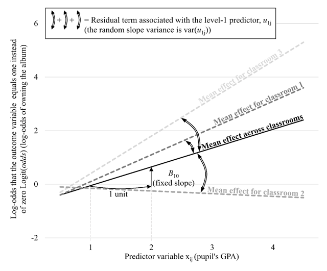
Figure 5
Graphical representation of the fixed slope B10 and the residual term associated with the level-1 predictor u1j (cf. Eq. 5); the fixed slope B10 corresponds to the overall effect of pupil’s GPA on the log-odds of owning Justin’s album across classrooms; the random intercept variance var(u0j) corresponds to the variance of the deviation of the classroom-specific effects of pupil’s GPA from the overall effect of pupil’s GPA (here represented by the double-headed arrow for the 1st, 2nd, and 3rd classroom). Notes: Data are fictitious and do not correspond to the provided dataset.
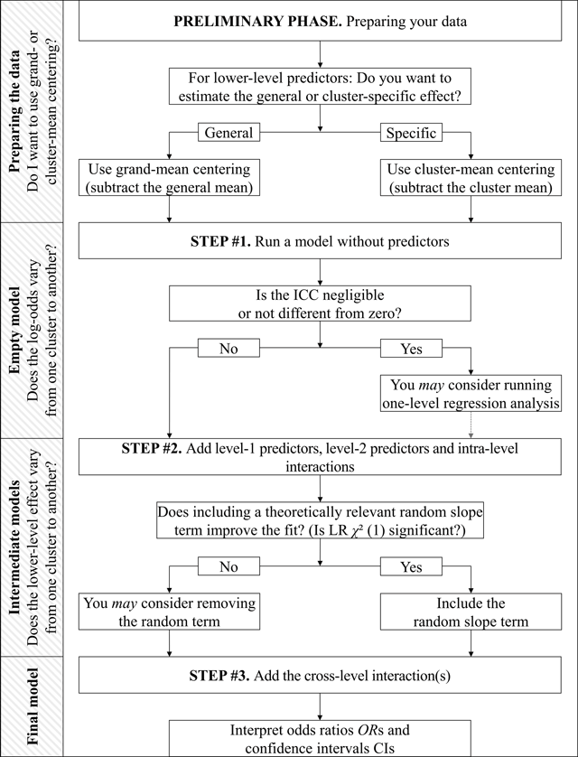
Figure 6
Summary of the three-step simplified procedure for multilevel logistic regression.