

Figure 1
The 8 × 10 hand signed photo of the great Justin Timberlake that YOU could win (upper panel), along with its numbered hologram Certificate of Authenticity (lower panel).
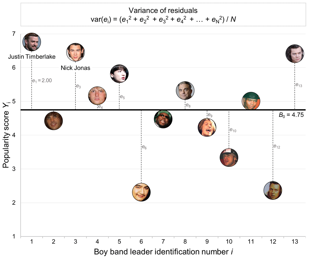
Figure 2
Graphical representation of a linear regression with no predictor (Eq. 2) in which the observed popularity score Yi (y-axis) of a particular boy band leader i (x-axis) corresponds to the mean popularity score B0 (horizontal thick line) plus the residuals ei (vertical dotted lines). Notes: Only the first 13 observations are represented; despite the controversial fact that there is no official leader in One Direction, we treated Harry Styles as their boy band leader.
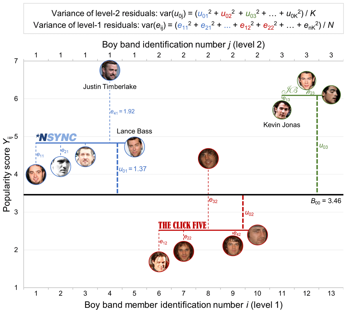
Figure 3
Graphical representation of a two-level linear regression with no predictor (Equation 4) in which the observed popularity score Yij (y-axis) of a particular boy band member i (bottom x-axis) from a particular boy band j (top x-axis) corresponds to the overall mean popularity score B00 (horizontal thick line) plus the level-2 residuals u0j (vertical thick dotted lines) and level-1 residuals eij (vertical thin dotted lines). Notes: Only the first 13 observations are represented; normally, B00 is only equivalent to the arithmetic grand-mean when the design is completely balanced (i.e., when the number of participants is the same for each cluster); the first author is somewhat prosopagnosic and apologizes in advance if he has erroneously interchanged two faces.
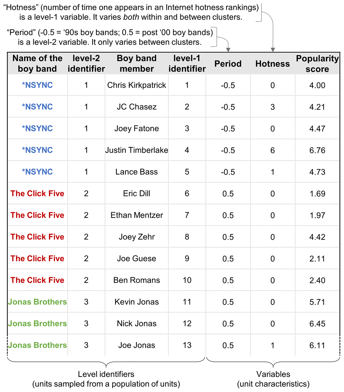
Figure 4
The 13 first lines of your boy band datasets. Notes: Fans often argue that ‘The Click Five’ is a pop rock band, not a boy band; we respectfully disagree with them, and we invite readers to watch The Click Five’s video clip ‘Kidnap My Heart’ on YouTube and make up their own mind (this song does not count as a hidden song).
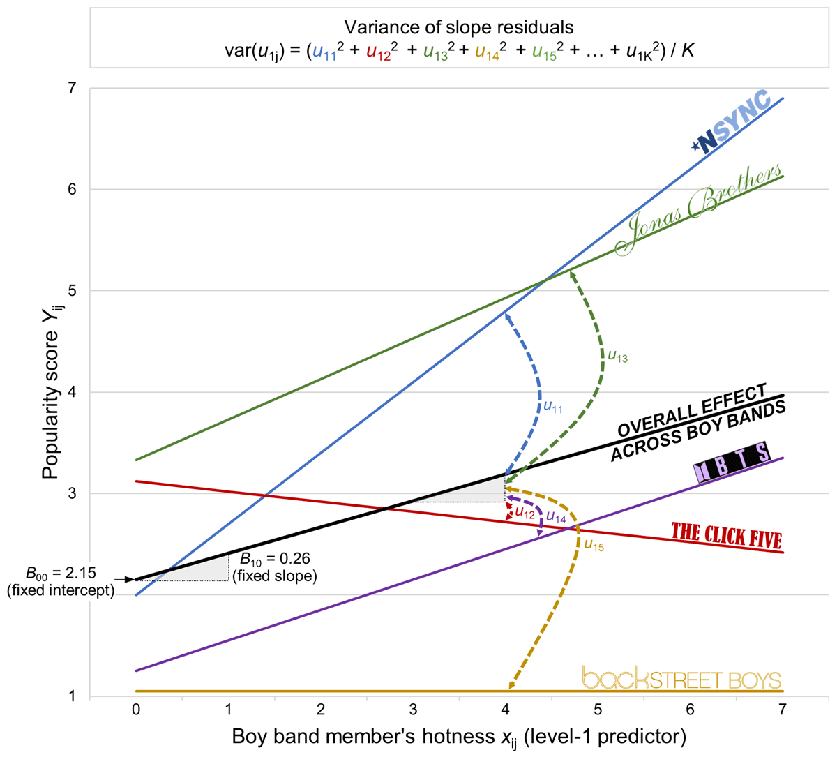
Figure 5
Graphical representation of the coefficient estimate or fixed slope B10 (the thick slope – the overall mean effect of hotness across boy bands) and the slope residuals u1j (vertical thick dotted curves – the differences between the specific effects of hotness in a given boy band compared to the overall mean effect). Notes: Only the first five boy bands are represented; obviously, the data for this figure are fictitious (the Backstreet Boys are still way more popular than that!).
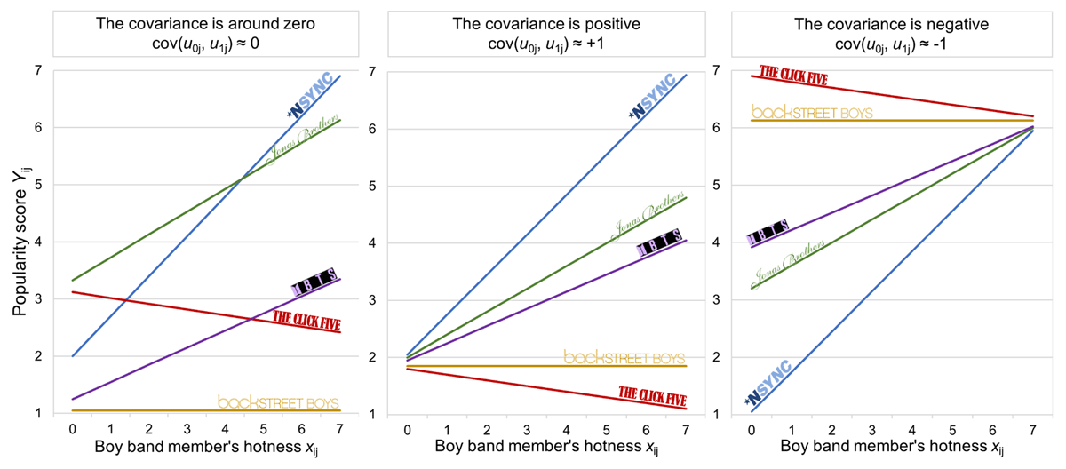
Figure 6
Graphical representations of the covariance between the intercept residuals (or level-2 residuals) u0j and the slope residuals u1j. In the left panel, the covariance is equal to zero (no pattern), in the middle panel, the covariance is positive (higher boy band-specific intercepts come with larger slopes), and in the right panel, the covariance is negative (higher boy band-specific intercepts come with smaller slopes). Note: Again, the data for this figure are fictitious.
Table 1
Summary of the main notations and definitions of two-level modeling concepts.
| Level 2 K level-2 units (clusters) with n observations per cluster (mean cluster size) | Level 1 N level-1 units (observations) | |
|---|---|---|
| The first principle: Two types of residuals | u0j Level-2 residuals or intercept residuals (“random intercept”) Distance of the cluster-specific means from the overall mean Tip: The aggregated index of level-2 residuals is var(u0j) | eij Level-1 residuals Distance of the observations from the cluster-specific means Tip: The aggregated index of level-1 residuals is var(eij) |
| The second principle: Two types of variable | X1j, X2j,
X3j, etc. Level-2 predictors Cluster characteristics Tip: They CANNOT vary within clusters | x1ij, x2ij,
x3ij, etc. Level-1 predictors Observation characteristics Tip: They CAN vary within clusters |
| The third
principle: Two types of level-1 effects parameters | B00,
B01, B02,
B03, etc. Fixed intercept (B00) and level-2 coefficient estimates (B01…) Overall mean/intercept and effects of X1ij, X2ij, X3ij, etc. | B10,
B20, B30,
etc. Level-1 coefficient estimates or fixed slopes Overall mean effect of x1ij, x2ij, x3ij, etc., across all clusters |
| N/a Slope residuals are not possible for level-2 predictors | u1j,
u2j, u3j,
etc. Variation of the effect of the level-1 predictors orslope residuals (“random slopes”) Differences between the cluster-specific slopes and the fixed slope Tip 1: The variance term is var(u1j), var(u2j), etc. Tip 2: The covariance term is cov(u0j, u1j), etc. |
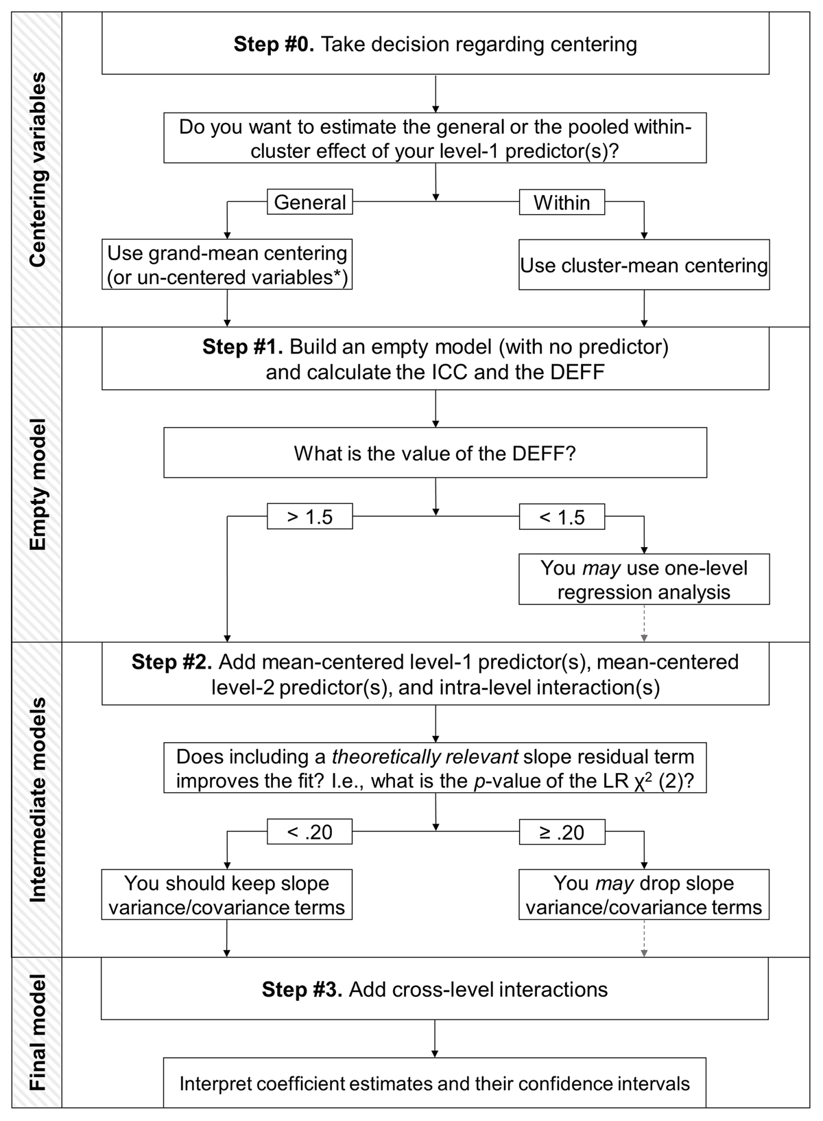
Figure 7
Decision tree illustrating the three-step procedure for two-level linear modeling. Note: *We recommend always centering your predictor when your model includes an interaction term.
Table 2
Convergence rates, slope residual variance detection rates, type II (when β11 ≥ 0.05) and type I (when β11 = 0.00) error rates as a function of the statistical software (SPSS vs. Stata vs. R vs. Mplus), the size of the cross-level interaction (small vs. very small vs. zero), and the magnitude of the slope residuals variance (small vs. very small vs. near zero).
| # | Condition 3 × 3 | Convergence rates Proportion of models, in 100 iterations | Slope residual variance detection rates Proportion of sig. LR χ² with α = 0.20 | Type II and type I error rates Proportion of [non]sig. B11 with α = 0.05 | |||||||||||
|---|---|---|---|---|---|---|---|---|---|---|---|---|---|---|---|
| Interaction(β11) | Residuals(var(u1j)) | SPSS | Stata | R | Mplus | SPSS | Stata | R | Mplus | SPSS | Stata | R | Mplus | ||
| 1. | Small (0.10) | Small (0.01) | 1.00 [1.0, 1.0] | 1.00 [1.0, 1.0] | .97 [0.96, 0.98] | 1.00 [1.0, 1.0] | 1.00 [1.0, 1.0] | 1.00 [1.0, 1.0] | 1.00 [1.0, 1.0] | 1.00 [1.0, 1.0] | 0.21 [0.19, 0.24] | 0.20 [0.17, 0.22] | 0.20 [0.17, 0.22] | 0.20 [0.17, 0.23] | Type II error |
| 2. | Small (0.10) | Very small (0.005) | 1.00 [1.0, 1.0] | 1.00 [1.0, 1.0] | 0.98 [0.97, 0.99] | 1.00 [1.0, 1.0] | 1.00 [1.0, 1.0] | 1.00 [1.0, 1.0] | 1.00 [1.0, 1.0] | 1.00 [1.0, 1.0] | 0.07 [0.05, 0.08] | 0.06 [0.05, 0.08] | 0.06 [0.05, 0.08] | 0.06 [0.05, 0.08] | |
| 3. | Small (0.10) | Near zero (0.001) | 0.89 [0.87, 0.91] | 0.99 [0.98, 0.99] | 0.98 [0.97, 0.99] | 1.00 [1.0, 1.0] | 0.99 [1.0, 1.0] | 0.99 [1.0, 1.0] | 0.99 [1.0, 1.0] | 0.99 [1.0, 1.0] | 0.00 [0.00, 0.01] | 0.00 [0.00, 0.01] | 0.00 [0.00, 0.01] | 0.00 [0.00, 0.01] | |
| 4. | Very small (0.05) | Small (0.01) | 1.00 [1.0, 1.0] | 1.00 [1.0, 1.0] | 0.98 [0.97, 0.99] | 1.00 [1.0, 1.0] | 1.00 [1.0, 1.0] | 1.00 [1.0, 1.0] | 1.00 [1.0, 1.0] | 1.00 [1.0, 1.0] | 0.73 [0.70, 0.75] | 0.70 [0.67, 0.73] | 0.70 [0.67, 0.73] | 0.70 [0.67, 0.73] | |
| 5. | Very small (0.05) | Very small (0.005) | 1.00 [1.0, 1.0] | 1.00 [1.0, 1.0] | 0.99 [0.98, 0.99] | 1.00 [1.0, 1.0] | 1.00 [1.0, 1.0] | 1.00 [1.0, 1.0] | 1.00 [1.0, 1.0] | 1.00 [1.0, 1.0] | 0.57 [0.54, 0.60] | 0.55 [0.52, 0.58] | 0.55 [0.52, 0.58] | 0.55 [0.52, 0.58] | |
| 6. | Very small (0.05) | Near zero (0.001) | 0.90 [0.87, 0.91] | 0.99 [0.98, 1.0] | 0.98 [0.97, 0.99] | 1.00 [1.0, 1.0] | 0.81 [0.85, 0.83] | 0.81 [0.85, 0.83] | 0.81 [0.86, 0.83] | 0.81 [0.85, 0.83] | 0.25 [0.22, 0.28] | 0.23 [0.20, 0.26] | 0.23 [0.20, 0.26] | 0.23 [0.21, 0.26] | |
| 7. | Zero (0.00) | Small (0.01) | 1.00 [1.0, 1.0] | 1.00 [1.0, 1.0] | 0.98 [0.97, 0.99] | 1.00 [1.0, 1.0] | 1.00 [1.0, 1.0] | 1.00 [1.0, 1.0] | 1.00 [1.0, 1.0] | 1.00 [1.0, 1.0] | 0.03 [0.02, 0.04] | 0.03 [0.02, 0.04] | 0.03 [0.02, 0.04] | 0.03 [0.02, 0.04] | Type I error |
| 8. | Zero (0.00) | Very small (0.005) | 1.00 [1.0, 1.0] | 1.00 [1.0, 1.0] | 0.98 [0.97, 0.99] | 1.00 [1.0, 1.0] | 0.99 [1.0, 1.0] | 0.99 [1.0, 1.0] | 0.99 [1.0, 1.0] | 0.99 [1.0, 1.0] | 0.03 [0.02, 0.04] | 0.03 [0.02, 0.05] | 0.03 [0.02, 0.05] | 0.03 [0.02, 0.05] | |
| 9. | Zero (.00) | Near zero (.001) | 0.88 [0.86, 0.90] | 0.99 [0.99, 1.0] | 0.97 [0.96, 0.98] | 1.00 [1.0, 1.0] | 0.53 [0.60, 0.56] | 0.53 [0.60, 0.56] | 0.54 [0.60, 0.57] | 0.53 [0.60, 0.56] | 0.02 [0.01, 0.03] | 0.02 [0.01, 0.03] | 0.02 [0.01, 0.03] | 0.02 [0.01, 0.03] | |
[i] Notes: 95% CIs are given in brackets.