

Figure 1
A subak meeting in a Balinese village. Although the Balinese language includes registers (high and low) connected with the relative caste status of the speaker and hearer, during these meetings the registers are set aside and all participants are strongly encouraged to speak in the same register, signalling their equal status in the subak. See text for analysis of the consequences for governance.
Table 1
Survey topics used in this study. The 19 questions used in the reduced list for analysis are highlighted. The use of higher order clustering to reduce the number of descriptors from 35 to 19 is explained in SI B.
| DESCRIPTOR # | DESCRIPTOR | DESCRIPTOR # | DESCRIPTOR |
|---|---|---|---|
| 1 | Own farmland | 19 | Pest damage in subak |
| 2 | Sharecrop land | 20 | Pest damage myself |
| 3 | Inherited a farm | 21 | Thefts of water |
| 4 | Purchase | 22 | Conflicts among members |
| 5 | Sold a farm | 23 | Choice of subak head |
| 6 | Income | 24 | Fines |
| 7 | Harvest | 25 | Crop schedule followed |
| 8 | Satisfaction with harvest | 26 | Plan work |
| 9 | Origin | 27 | Written rules followed |
| 10 | Condition of canals | 28 | Fines frequency |
| 11 | Condition of fields | 29 | Condition of subak |
| 12 | Synchronize | 30 | Decisions of subak accepted |
| 13 | Attendance at meetings | 31 | Technical problems |
| 14 | Participation in maintenance | 32 | Social problems |
| 15 | Attendance at ritual | 33 | Caste problems |
| 16 | Accept subak decisions | 34 | Class problems |
| 17 | Water shortages in subak | 35 | Resilience |
| 18 | Water shortages myself |
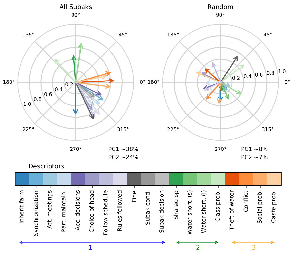
Figure 2
Comparison of PCA biplots of survey data from all 20 subaks, and from randomized samples as control. The randomized samples are obtained by shuffling the responses of all the farmers to each question independently, re-running the PCA, and calculating the biplot (see the Matlab codes section for a sample code used to plot the biplot). Each descriptor is assigned a unique color. The length of the arrow for each descriptor indicates its magnitude (contribution to the PCA). Arrows that are closer together are more correlated. Note that the direction of each arrow is relative to that of the descriptor “inherit farm” which is a fixed reference at 270° for both biplots. Blues, purples and greys are cooperative descriptors (1); greens are defective descriptors (2); and oranges are social disharmony descriptors (3).
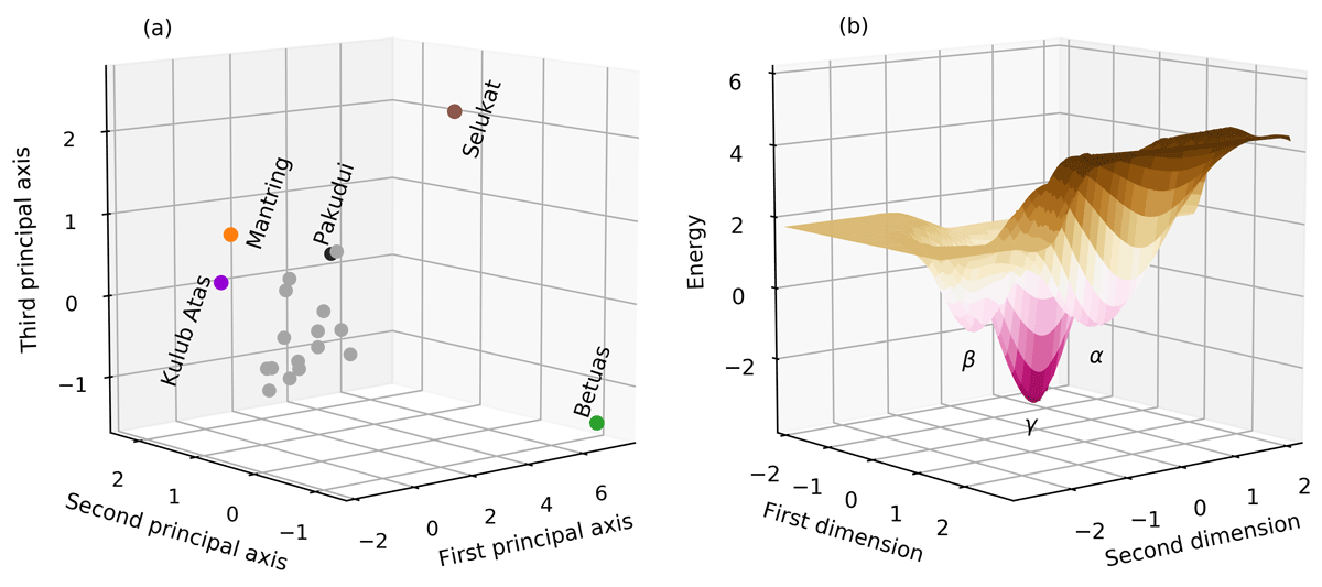
Figure 3
Analysis of the survey results shows that survey responses cluster at the subak level, indicating that certain combinations of attitudes are common. (a) PCA at the level of subaks rather than individual farmers shows one large cluster (grey) and 5 subaks that are outliers. 19 descriptors account for most of the variance (PC1 = 38%, PC2 = 24%, PC3 = 9.6%.). (b) Energy landscape analysis based on Fisher Information at the subak scale shows three attractors corresponding to the PCA clusters. The more cohesive the descriptors within a cluster, the denser the state and the greater the depth.
Table 2
Parameter values for each subak for the Steering Capacity equation. See Section F of SI for variables.
| SUBAK NUMBER # | NAME | VARIABLES | ||
|---|---|---|---|---|
| B | D | T | ||
| 1 | Tampuagan Hilir | 0 | 1 | 25 |
| 2 | Mantring | 13 | 7 | 42 |
| 3 | Tampuagan Hulu | 1 | 0 | 9 |
| 4 | Kebon | 0 | 0 | 64 |
| 5 | Calo | 0 | 0 | 52 |
| 6 | Cebok | 0 | 0 | 51 |
| 7 | Bayad | 0 | 0 | 60 |
| 8 | Timbul | 0 | 0 | 47 |
| 9 | Kedisan kaja | 0 | 0 | 38 |
| 10 | Kedisan Kelod | 0 | 0 | 38 |
| 11 | Jasan | 0 | 1 | 32 |
| 12 | Selukat | 0 | 14 | 10 |
| 13 | Sebatu | 0 | 0 | 52 |
| 14 | Betuas | 71 | 16 | 24 |
| 15 | Pakudui | 0 | 8 | 19 |
| 16 | Aban | 0 | 1 | 37 |
| 17 | Teba | 1 | 1 | 45 |
| 18 | Dukuh | 23 | 1 | 28 |
| 19 | Tegan | 4 | 2 | 64 |
| 20 | Kulub Atas | 4 | 3 | 90 |
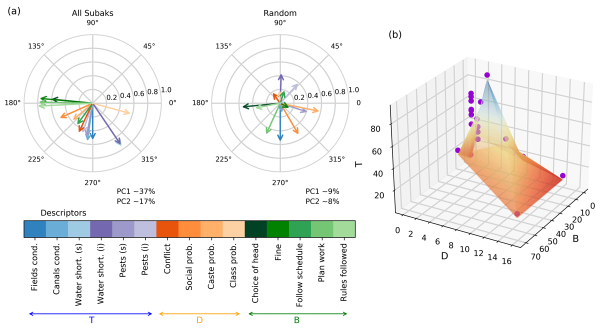
Figure 4
Relationship of perceived environmental threats T to the suppression of social dominance behavior D and breakdowns in consensus-based collective decision-making B based on surveys of 496 farmers in 20 Balinese subaks. These variables are a subset of the full set in Figure 1 and have different colors. The greater the threat T (based on the mean of 7 variables), the fewer breakdowns in collective management by the subak B (4 variables), and the less dominance-related behavior D (4 variables). Left: Principal Components analysis of responses to the survey questions that define T, B and D. These are a subset of the variables (see Figure 1). The length of each vector arrow is proportional to the statistical significance of a survey question, and its direction is proportional to its correlation with other survey questions. Right: Each dot represents aggregate survey results for a single subak. At low levels of threat (T), both B and D are present in some subaks. As T increases, B and D rapidly decline. We interpret this to mean that as perceived environmental threats to the group increase, obstacles to effective collective decision making (steering capacity) are suppressed.

Figure 5
Steering capacity model with colours for the three different attractors. Attractor α is red (subaks Betuas and Selukat), Attractor β is blue (subaks Kulub Atas and Mantring); the remaining 16 subaks in Attractor γ are black. Note that the observables T, D and B are to be treated as independent variables in SC = f(T,–D,–B), which expresses the generic feature of steering capacity as a quantity that increases with perceived environmental threat, and decreases under social dominance behaviour as well as breakdown in consensus based collective decision-making. Thus these figures should not be interpreted as a relationship between T, D and B. Instead the figure shows that subaks with high T, low D, and low B (black dots) have high steering capacity; and those with relatively low T and relatively high D and B (red and blue dots) have a relatively lower steering capacity.
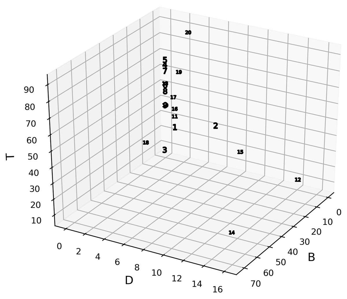
Figure 6
Steering capacity model with numbered subaks in the attractors. Attractor α includes 14 Betuas and 12 Selukat; Attractor β includes 20 Kulub Atas and 2 Mantring. 15 Pakudu is an interesting outlier in Attractor γ, see text. See table 2 for parameter values based on the 19 variables used for analysis.

Figure 7
Fisher Information landscape showing clustering of survey responses at the subak level. Here, we project survey answers of the 493 farmers onto the first two principal components, and calculate the density of the population in the principal component space. The density of a state is defined as the number of subaks per state (See Methods and SI). Most of the farmers lie at the centre of the blue rings, which enclose the survey responses from subaks in Attractor γ, which we interpret as exhibiting high steering capacity. Colored dots show the responses of individual farmers in subaks in Attractor α and Attractor β, which are both more divergent and less cohesive than Attractor γ, with lower Fisher Information. As noted in the text, the steering capacity of #15 Pakudui, which lies within Attractor γ, is being tested by social conflicts extrinsic to the subak itself.
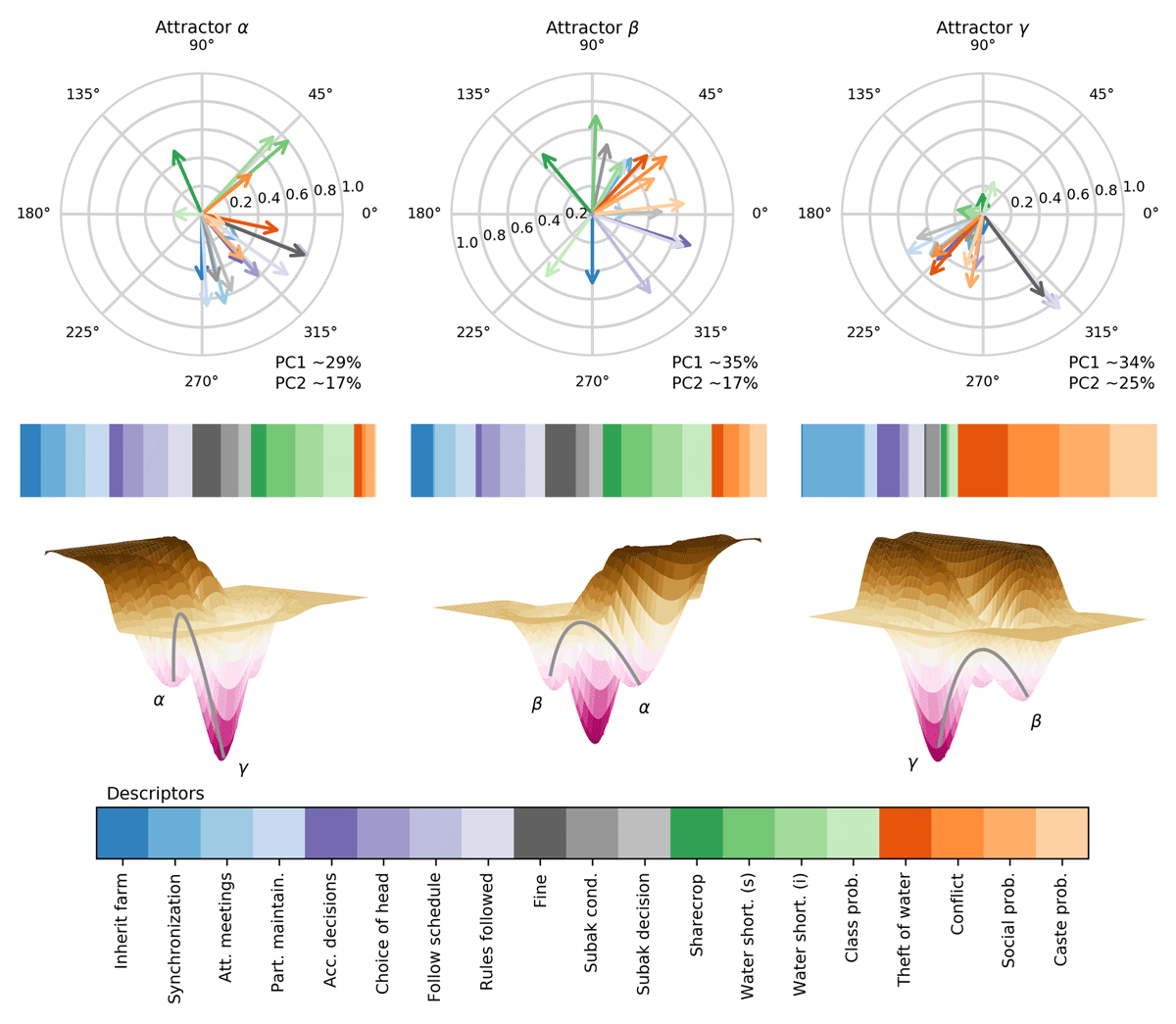
Figure 8
Transition paths between the regimes calculated from the energy landscape analysis. Equation 1 predicts different solutions for each regime, each of them nearly linear within that regime, because the correlations among variables are different for each regime. The top panel shows the biplots for the three regimes. The direction of each arrow of the biplots is relative to that of the descriptor “inherit farm” which is a fixed reference at 270°. Attractor α includes Subaks Betuas and Selukat; Attractor β consists of Mantring and Kulub Atas; all other subaks are in Attractor γ. Below this panel, the colored band shows which descriptors dominate along hypothetical transition paths between regimes (attractors). Environmental variables (in green) and fines dominate the path from α to γ, but have little influence on the path from β to γ, which is dominated by social conflicts (in red). Thus a reduction in environmental problems would lead a transition from α to γ, while reduction in social conflicts would lead from β to γγ. The third panel shows the energy landscape and these transition paths. Beneath it the colored band shows all 19 descriptors.
Table 3
Loading Matrix of the 19 descriptors for energy landscape analysis.
| DESCRIPTOR # | DESCRIPTOR | COMPONENTS | ||
|---|---|---|---|---|
| 1 | 2 | 3 | ||
| 3 | Inherited a farm | –0.6758 | 0.4621 | 0.2448 |
| 12 | Synchronize | –0.8662 | –0.1861 | –0.1163 |
| 13 | Attendance at meetings | –0.8429 | 0.0664 | 0.0860 |
| 14 | Participation in maintenance | –0.8938 | –0.0684 | 0.0717 |
| 16 | Accept subak decisions | –0.7376 | –0.2356 | 0.2600 |
| 23 | Choice of subak head | –0.8230 | 0.0847 | 0.0655 |
| 26 | Plan work | –0.9670 | 0.1173 | 0.0815 |
| 27 | Written rules followed | –1.0031 | 0.0031 | 0.0231 |
| 24 | Fines | 0.1244 | 0.0431 | 0.0317 |
| 29 | Condition of subak | –0.6587 | –0.0983 | –0.0828 |
| 30 | Decision of subak accepted | –0.6433 | –0.0232 | 0.4136 |
| 2 | Sharecrop land | 0.6190 | –0.3588 | –0.2771 |
| 17 | Water shortages in subak | 0.7361 | –0.6646 | 0.2997 |
| 18 | Water shortages myself | 0.7519 | –0.6666 | 0.2749 |
| 34 | Class problems | 0.8679 | 0.0026 | 0.3283 |
| 21 | Theft of water | –0.6333 | –0.6276 | 0.0693 |
| 22 | Conflicts among members | –0.4316 | –0.6765 | 0.0407 |
| 32 | Social problems | –0.7157 | –0.4868 | –0.2364 |
| 33 | Caste problems | –0.4227 | –0.5815 | –0.2555 |