
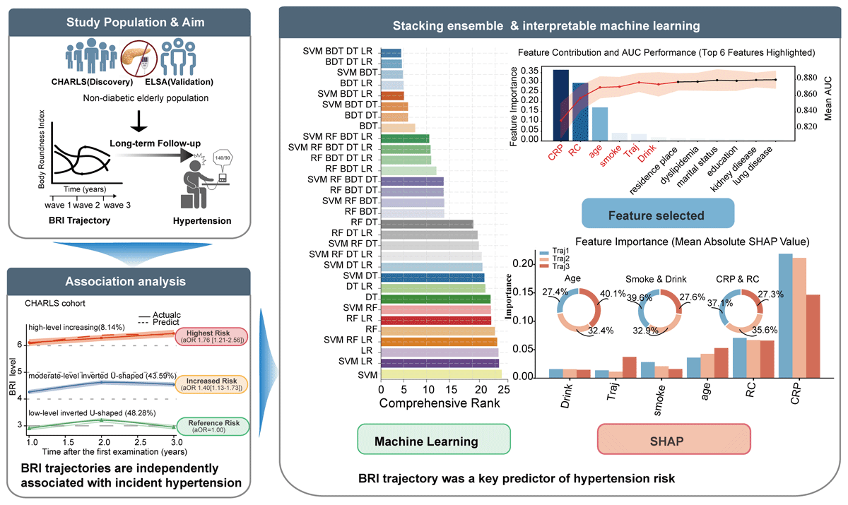
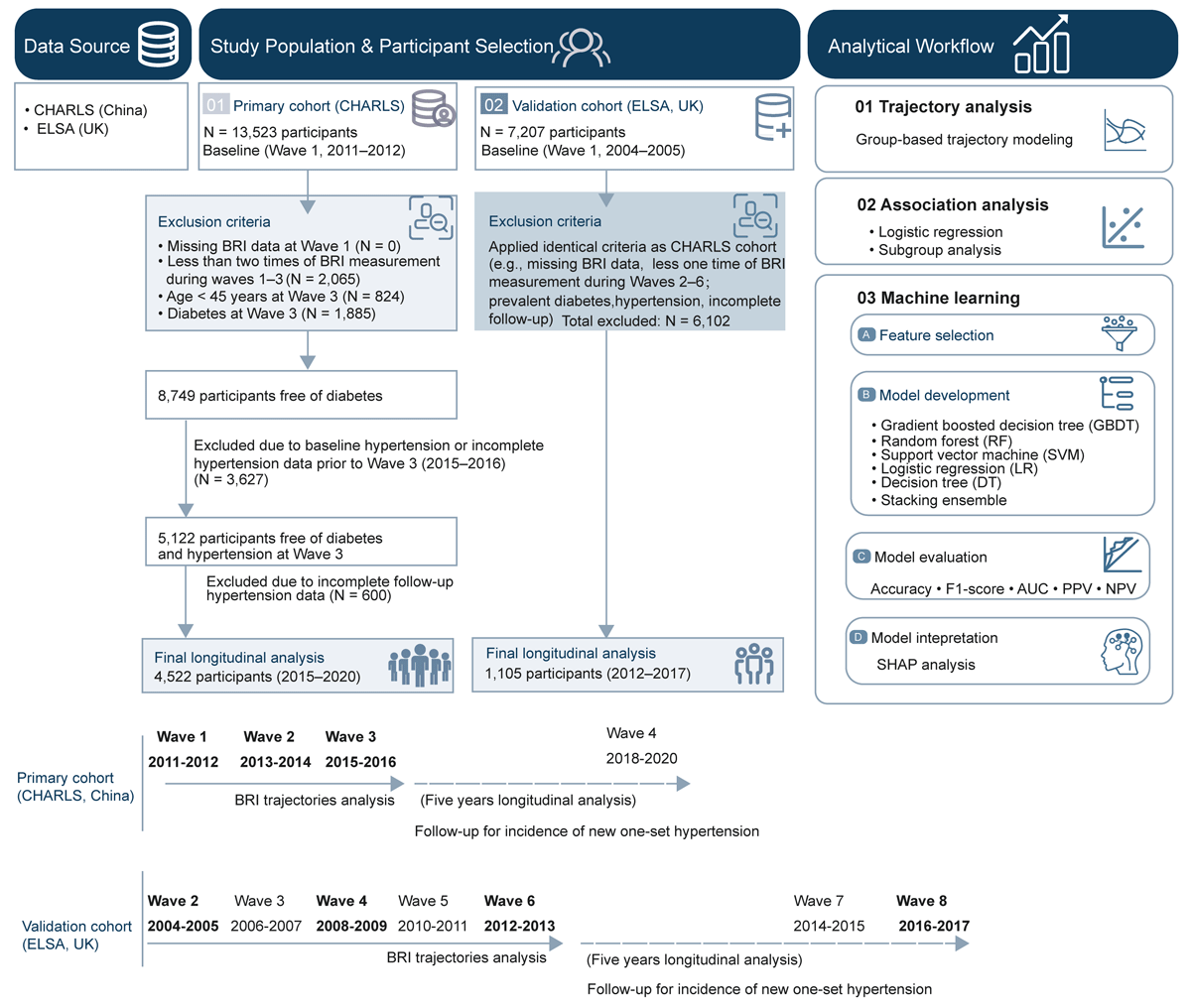
Figure 1
Study design, participant selection, and analytical workflow.
Table 1
Evaluation index of optimal trajectory model.
| TRAJECTORY GROUP | SHAPE | AVEPP% | n | (Pj) | (πj) | OCC | Ej |
|---|---|---|---|---|---|---|---|
| Group1 | Quadratic | 89.06 | 2183 | 48.28 | 47.91 | 8.8 | 0.732 |
| Group2 | Quadratic | 85.23 | 1971 | 43.59 | 43.47 | 7.5 | |
| Group3 | Linear | 87.17 | 368 | 8.14 | 8.62 | 72.0 |
[i] Avepp, average posterior probability; Pj, estimated group membership probability; πj, observed group proportion; OCC, odds of correct classification; Ej, classification error index.
Table 2
Baseline characteristics of the study population according to BRI trajectory.
| VARIABLE | TOTAL (n = 4,522) | TRAJ 1 (n = 2,183) | TRAJ 2 (n = 1,971) | TRAJ 3 (n = 368) | STATISTIC | p-value* |
|---|---|---|---|---|---|---|
| Age | 60.29 ± 8.51 | 60.59 ± 8.45 | 59.87 ± 8.54 | 60.81 ± 8.64 | 4.46 | 0.01 |
| Body mass index | 22.74 ± 3.28 | 20.80 ± 2.30 | 24.01 ± 2.57 | 27.51 ± 3.52 | 1536.34 | <0.0001 |
| Sex | 405.82 | <0.0001 | ||||
| female | 2458(54.36) | 868(39.76) | 1282(65.04) | 308(83.70) | ||
| male | 2064(45.64) | 1315(60.24) | 689(34.96) | 60(16.30) | ||
| Marital status | 1.77 | 0.41 | ||||
| married | 4022(88.94) | 1955(89.56) | 1744(88.48) | 323(87.77) | ||
| other | 500(11.06) | 228(10.44) | 227(11.52) | 45(12.23) | ||
| Residence place | 30.67 | <0.0001 | ||||
| rural | 3104(68.64) | 1584(72.56) | 1287(65.30) | 233(63.32) | ||
| urban | 1418(31.36) | 599(27.44) | 684(34.70) | 135(36.68) | ||
| Education | 3.17 | 0.20 | ||||
| High school or above | 479(10.59) | 234(10.72) | 216(10.96) | 29 (7.88) | ||
| Middle school and below | 4043(89.41) | 1949(89.28) | 1755(89.04) | 339(92.12) | ||
| Drink | 120.82 | <0.0001 | ||||
| no | 2962(65.50) | 1267(58.04) | 1394(70.73) | 301(81.79) | ||
| yes | 1560(34.50) | 916(41.96) | 577(29.27) | 67(18.21) | ||
| Smoke | 335.23 | <0.0001 | ||||
| Never | 2692(59.53) | 1026(47.00) | 1353(68.65) | 313(85.05) | ||
| Former smoker | 535(11.83) | 290(13.28) | 226(11.47) | 19 (5.16) | ||
| Current smoker | 1295(28.64) | 867(39.72) | 392(19.89) | 36 (9.78) | ||
| Stroke | 3.71 | 0.16 | ||||
| no | 4458(98.58) | 2151(98.53) | 1948(98.83) | 359(97.55) | ||
| yes | 64 (1.42) | 32 (1.47) | 23 (1.17) | 9 (2.45) | ||
| Dyslipidemia | 120.91 | <0.0001 | ||||
| no | 3454(76.38) | 1821(83.42) | 1393(70.67) | 240(65.22) | ||
| yes | 1068(23.62) | 362(16.58) | 578(29.33) | 128(34.78) | ||
| Lung disease | 4.77 | 0.09 | ||||
| no | 3941(87.15) | 1878(86.03) | 1739(88.23) | 324(88.04) | ||
| yes | 581(12.85) | 305(13.97) | 232(11.77) | 44(11.96) | ||
| Cancer | 0.11 | 0.95 | ||||
| no | 4467(98.78) | 2157(98.81) | 1946(98.73) | 364(98.91) | ||
| yes | 55 (1.22) | 26 (1.19) | 25 (1.27) | 4 (1.09) | ||
| Kidney disease | 0.94 | 0.63 | ||||
| no | 4114(90.98) | 1977(90.56) | 1802(91.43) | 335(91.03) | ||
| yes | 408 (9.02) | 206 (9.44) | 169 (8.57) | 33 (8.97) | ||
| Heart disease | 13.42 | <0.01 | ||||
| no | 4035(89.23) | 1983(90.84) | 1737(88.13) | 315(85.60) | ||
| yes | 487(10.77) | 200 (9.16) | 234(11.87) | 53(14.40) | ||
| Incident hypertension | 38.21 | <0.0001 | ||||
| no | 3838(84.87) | 1920(87.95) | 1633(82.85) | 285(77.45) | ||
| yes | 684(15.13) | 263(12.05) | 338(17.15) | 83(22.55) |
[i] *ANOVA, the Kruskal-Wallis test, and the Chi-square test assume independence of observations. Traj, trajectory.
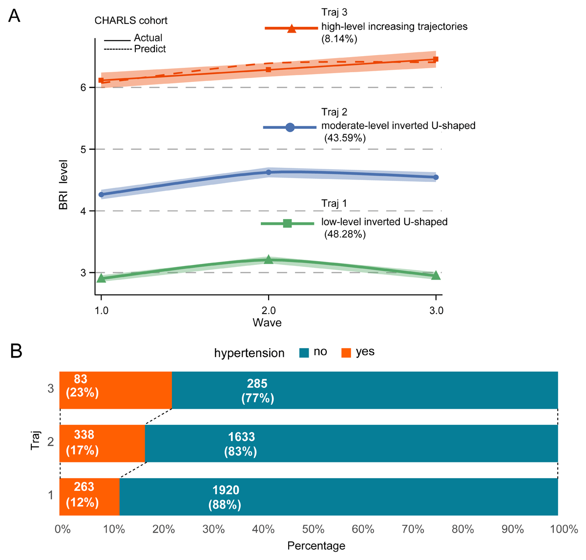
Figure 2
Longitudinal trajectories of body roundness index and incidence of hypertension in the CHARLS cohort. (A) Three-group BRI trajectory model. (B) Incidence of hypertension according to trajectory group.
Table 3
Association between trajectories of BRI and new-onset hypertension risk.
| CHARACTER | CRUDE MODEL | MODEL 1 | MODEL 2 | MODEL 3 | ||||
|---|---|---|---|---|---|---|---|---|
| OR (95%CI) | P | OR (95%CI) | P | OR (95%CI) | P | OR (95%CI) | P | |
| Trajectory | ||||||||
| 1 | ref | ref | ref | ref | ||||
| 2 | 1.51(1.27,1.80) | <0.0001 | 1.57(1.31,1.88) | <0.0001 | 1.39(1.13,1.72) | 0.002 | 1.40(1.13,1.73) | 0.002 |
| 3 | 2.13(1.61,2.80) | <0.0001 | 2.21(1.66,2.95) | <0.0001 | 1.77(1.22,2.56) | 0.003 | 1.76(1.21,2.56) | 0.003 |
| p for trend | <0.0001 | <0.0001 | <0.001 | <0.001 | ||||
[i] Crude model includes only the trajectory of BRI variable; Model 1 was adjusted for age, sex, marital status, residence, and education; Model 2 was additionally adjusted for c-reactive protein, triglycerides, remnant cholesterol, smoking, and alcohol consumption; Model 3 was further adjusted for dyslipidemia, heart disease, stroke, kidney disease, and lung disease. OR (95%CI), odds ratios and 95% confidence intervals; BRI, body roundness index.
Table 4
Association between BRI trajectory and hypertension incidence in ELSA cohort.
| VARIABLE | CRUDE MODEL | MODEL 1 | MODEL 2 | MODEL 3 | ||||
|---|---|---|---|---|---|---|---|---|
| OR (95%CI) | P | OR (95%CI) | P | OR (95%CI) | P | OR (95%CI) | P | |
| Trajectory | ||||||||
| 1 | ref | ref | ref | ref | ||||
| 2 | 1.13(0.82,1.56) | 0.461 | 1.05(0.76,1.47) | 0.759 | 1.05(0.75,1.47) | 0.764 | 1.04(0.74,1.45) | 0.835 |
| 3 | 1.78(1.09,2.89) | 0.021 | 1.67(1.02,2.74) | 0.043 | 1.65(1.00,2.71) | 0.049 | 1.67(1.01,2.75) | 0.044 |
| p for trend | 0.042 | 0.101 | 0.109 | 0.112 | ||||
[i] Crude model includes only the trajectory of BRI variable; Model 1 was adjusted for age, sex, marital status, job, income and education; Model 2 was additionally adjusted for drink and smoking status; Model 3 was further adjusted for cancer, arrhythmia, and chronic obstructive pulmonary disease. BRI, body roundness index; OR (95%CI), odds ratios and 95% confidence intervals.
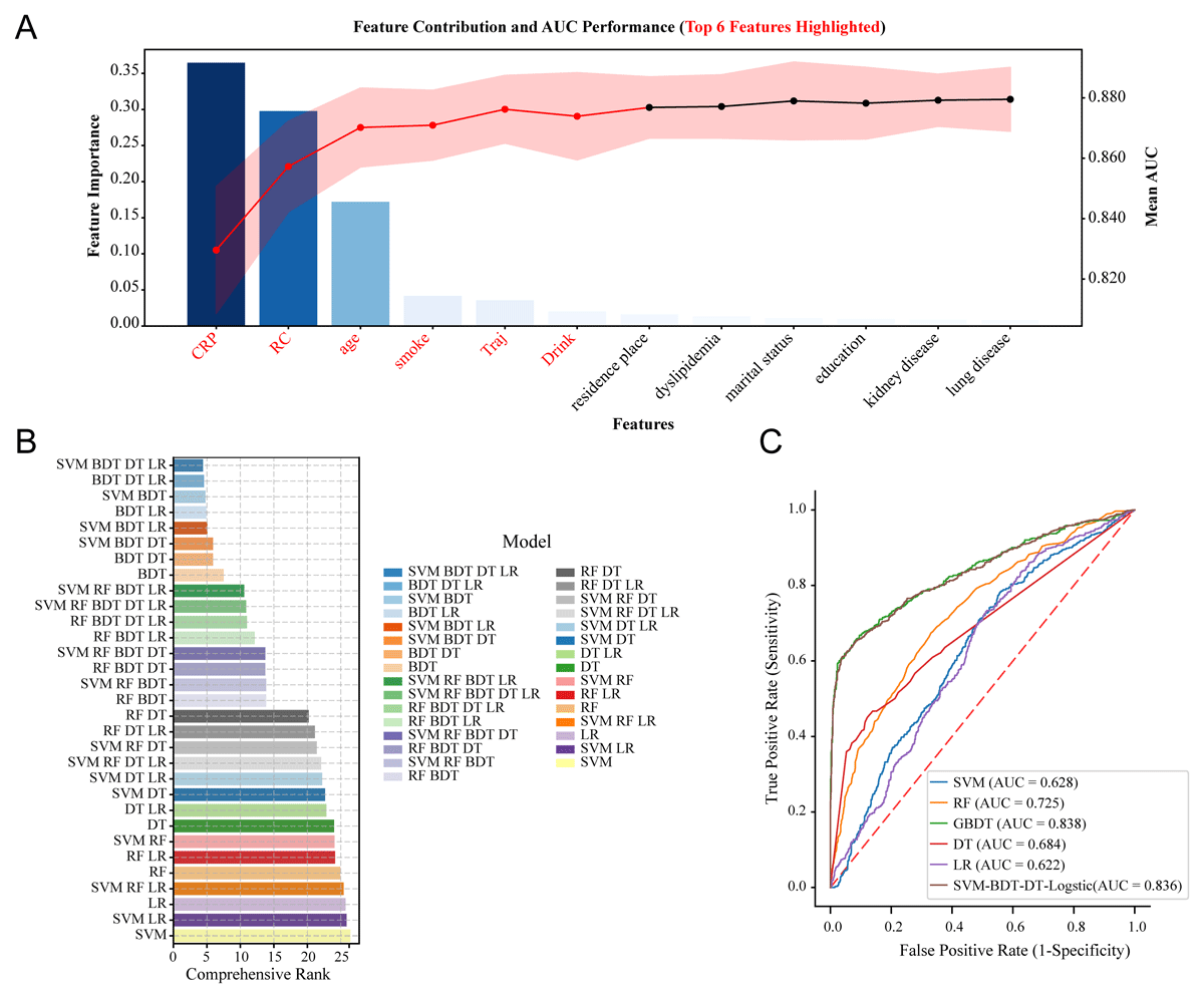
Figure 3
The comprehensive rank of five independent base ML models and various stacking ensemble combinations. (A) Features panel selection strategy implemented in the training set. Bars represent feature importance ranked by contribution to the prediction of incident hypertension. The line plot shows the cumulative area under the receiver operating characteristic curve (AUC; right y-axis) as features were sequentially added. Shaded areas indicate 95% confidence intervals estimated using 10-fold cross-validation. Features selected for the final model are highlighted in red and were identified based on the absence of significant incremental improvement in model performance over two consecutive iterations, as assessed by DeLong’s test (two-sided P > 0.05). (B) Comprehensive ranking of five individual machine learning models, random forest (RF), decision tree (DT), gradient boosting decision tree (GBDT), support vector machine (SVM), and logistic regression, and multiple stacking ensemble models in the testing set. The SVM–BDT–DT–Logistic stacking ensemble achieved the highest overall rank based on combined performance metrics. (C) Comparison of AUC values between the SVM–BDT–DT–Logistic stacking ensemble and individual machine learning models (RF, DT, GBDT, SVM, and logistic regression).
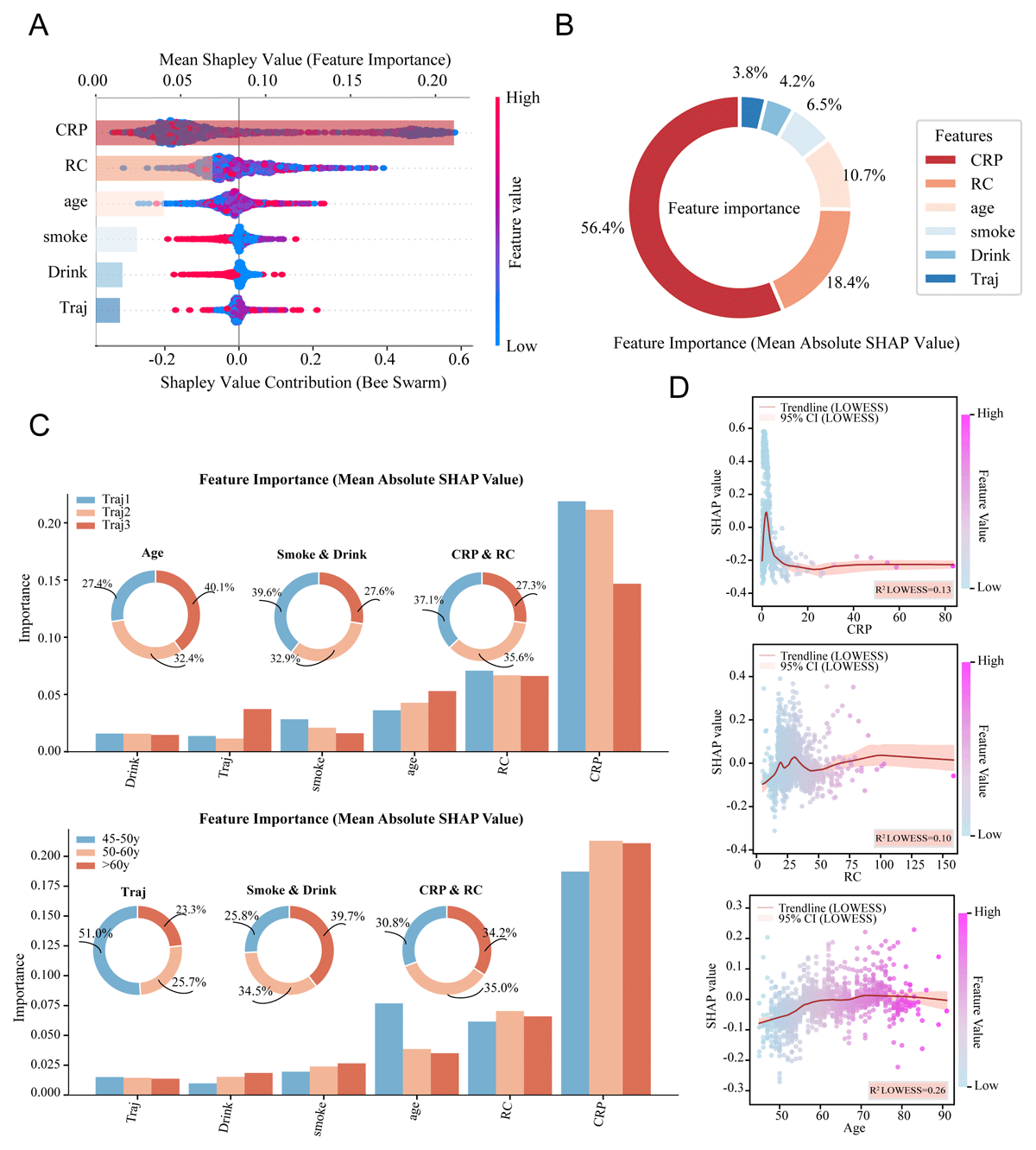
Figure 4
Global model interpretability analysis. (A) Combined SHAP summary and bar plots for the six features included in the hypertension risk prediction model. SHAP values represent the contribution of each feature to the model output. Each dot corresponds to an individual participant in the testing dataset and is colored according to the feature value, with vertical stacking indicating feature value density. The bar plot shows the mean absolute SHAP value for each feature. (B) Pie chart showing the relative percentage contribution of each of the six features to the prediction model, calculated based on the mean absolute SHAP values. (C) Bar plots and pie charts illustrating heterogeneity in feature contributions to the hypertension prediction model, quantified using SHAP values, across BRI trajectory groups (trajectory 1, trajectory 2, and trajectory 3) and age strata (45–50 years, 50–60 years, and >60 years). Feature groups include lifestyle factors (smoking and alcohol consumption) and biochemical markers (C-reactive protein and remnant cholesterol), with bars representing absolute contributions and pie charts indicating relative proportions. (D) SHAP dependence plots with locally weighted scatterplot smoothing (LOWESS) curves illustrating non-linear associations between continuous predictors (C-reactive protein, remnant cholesterol, and age) and model output. Each dot represents an individual participant, with SHAP values shown on the y-axis and corresponding feature values on the x-axis. The LOWESS curve summarizes the overall trend in feature contribution across the observed range of values.