
1. Introduction
The geomagnetic field as we see it today is the result of long-lasting, slowly varying processes occurring within the outer core and core mantle boundary. This field has a spatial variability due to the properties of Earth’s internal layers, such as changes in lithosphere and crust. An important implication of this field is shielding of the Earth’s atmosphere from the flow of continuous supersonic, massive solar wind. The understanding of geomagnetic field is essential to know the magnitude and frequency of extreme events like geomagnetic jerks and secular variation (Bharaswaj et al., 2013; Dumberry and Finlay, 2007; Finlay and Amit, 2011). These processes occur due to the internal sources of Earth’s magnetic field consisting of the primary field generated within the fluid outer core through geodynamo processes. Other processes that contribute to the spatial variability of magnetic field are lithospheric field, resulting from the superposition of induced and remnant magnetization in Earth’s subsurface rocks, along with contributions from oceanic circulation, tidal effects, and induction effects. The main magnetic field constitutes more than 99% of the magnetic field measured at the Earth’s surface. The remaining 1% portion is attributed to external sources originating in the magnetosphere and ionosphere, exhibiting temporal variations ranging from less than a few seconds to decades (Finlay et al., 2016). The dynamic interaction of solar wind with Earth’s magnetic field contributes to temporal variations on a broad range of time scales in both the external magnetospheric and ionospheric fields and their induced counterparts in Earth’s lithosphere and mantle (Campbell, 1997).
Global geomagnetic models have been developed using ground and satellite data sets. Few examples of global geomagnetic models are the CHAOS (Finlay et al., 2020), IGRF (Alken et al., 2021) and Comprehensive Models (Sabaka et al., 2020) families, among others. These models use the spherical harmonic analysis techniques and are continuously updated with more satellite and ground data sets. The primary source of station data for global magnetic field models involves observations from ground magnetometer networks from different parts of the world (INTERMAGNET and Super Mag are few examples). Observatories that contribute to these repositories often include only a few stations which may not give a correct picture of the regional based gridded magnetic field. For example, out of the available observatories across India, only three observatories (Jaipur (JAI), Alibag (ABG), operated by Indian Institute of Geomagnetism and Hyderabad (HYB), operated by CSIR- National Geophysical Research Institute) contribute to the refinement of these models. Although these models provide a holistic gridded map of the global magnetic field, the regional intricacies of magnetic fields are not resolved to a great extent. Especially, when the distribution of geomagnetic data is investigated in a small regional scale, it is important to invoke a regional based model, which allow a more accurate definition of the geomagnetic field in that region (Thébault et al., 2006; Nahayo et al., 2018; Nahayo and Korte, 2022).
The Revised Spherical Cap Harmonic Analysis (R-SCHA, Thébault et al., 2006) technique is the most recent regional based magnetic model developed using field measurements with altitude from ground to satellite as a spherical cone. This particular modelling technique has recently been applied in many regions of the world, such as Talarn et al. (2017) and Vervelidou et al. (2018). All these models use the mathematical formulation of spherical harmonic analysis to represent main magnetic field over any location. A pure data driven, regional based magnetic field model has not been developed so far and the current study aims at this science issue. In the pursuit of achieving this, we formulated a user-friendly MATLAB based GUI to obtain the gridded magnetic field using data at different geomagnetic observatories in the Indian region.
This 2D spatial grid of high resolution gridded magnetic field can help in understanding the regional changes in the magnetic field. The development of the gridded absolute and variation of magnetic field forms the central theme of this paper. In the subsequent sections, the data sets used, rigorous comparison among the interpolation methods, and details of GUI are provided.
2. Data
The geomagnetic field measurements were first initiated in 1841 with regular continuous measurement in 1846 by the Indian Institute of Geomagnetism (IIG) at Colaba, Mumbai, India. After the long records of more than a hundred years, IIG set up 12 geomagnetic observatories across the length and breadth of India for monitoring the continuous magnetic field measurements. While the data set itself is unique from 1980-to present, with a blend of absolute and variation types of magnetic measurements, it is useful for analyzing such geomagnetic extremes in the past as well. They are also useful for validating global magnetic field models and applications. IIG operates 12 geomagnetic observatories in India, where hourly (currently in second resolution) magnetic observations are recorded. Geomagnetic data for years in different volumes are being archived at the institute level. However, in this study, recent data from 11 observatories during 2011–2020 are used (excluding Port Blair) to validate and create the gridded geomagnetic map of India. Figure 1 includes the different geomagnetic observatories and period of geomagnetic data recordings. Table 1 lists the geographic and geomagnetic coordinates of all these stations. Most of these observatories were operating initially the IZMIRAN type of magnetic instruments, which were later replaced with Digital Flux gate magnetometers (DFM). The absolute measurements are taken at all the observatories using high precision Declination Inclination Magnetometer (DIM) and Proton Precision Magnetometer (PPM). These measurements are processed to compute respective baseline values and definitive data of one-minute resolution of the DFM system. These data are compiled, and quality is controlled and brought to a unified structures of the IAGA-2002 format. The temporal coverage of geomagnetic data recording at all these stations are different (as shown in Figure 1b). The maximum temporally covered and spatially available data sets are seen for the period of 2011–2020. Details of the data gaps during this period in included in Table S1. The data is subjected to basic quality checks like rejecting values, greater than exceeding known extreme values, breaks and jumps in the data etc. Unusual high values were flagged and are further examined for spatial continuity. Values showing spatial continuity are accepted and only the isolated values are rejected.
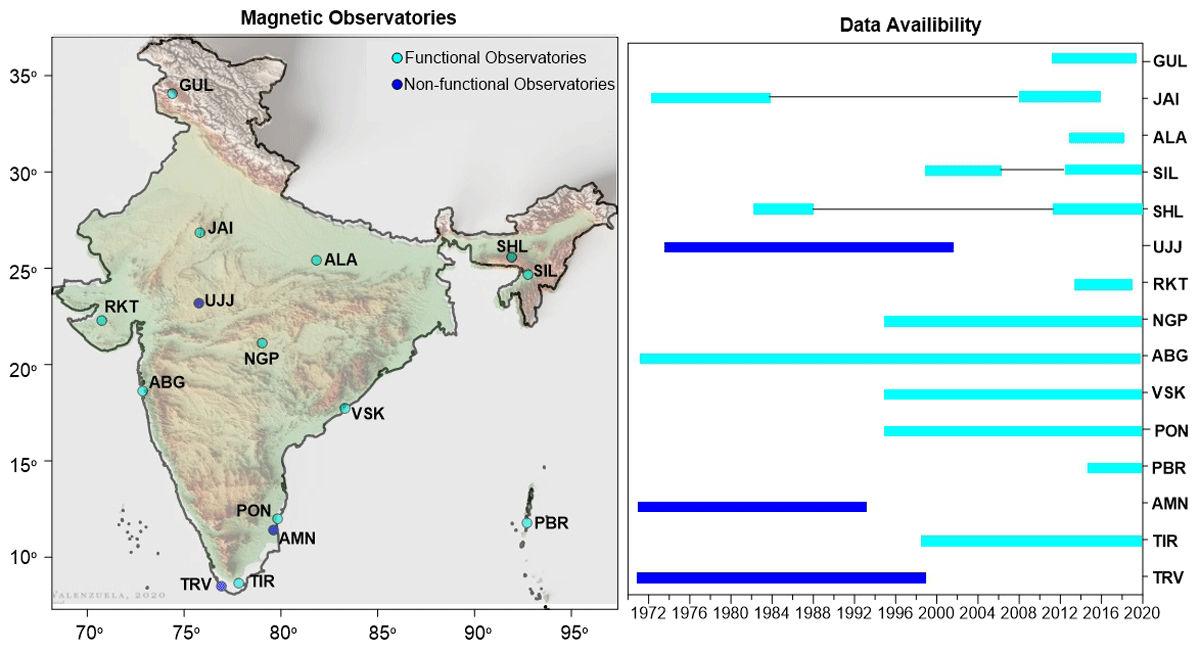
Figure 1
Location and Data availability of geomagnetic observations operated by Indian Institute of Geomagnetism. Station code abbreviations are included in Table 1.
Table 1
Location of geomagnetic observatories in India with station name, IAGA observatory code, type of instruments.
| S.NO. | MAGNETIC OBSERVATORY | IAGA CODE | INSTRUMENT TYPE | GEOGRAPHIC | GEOMAGNETIC |
|---|---|---|---|---|---|
| LATITUDE(N) LONGITUDE(E) | LATITUDE(N) LONGITUDE(E) | ||||
| 1. | Tirunelveli | TIR | Izmiran, DFM | 8° 42’ 77° 48’ | 0.15° 150.71° |
| 2. | Port Blair | PBR | DFM | 11° 48’ 92° 43’ | 2.28° 165.56° |
| 3. | Pondichery | PND | Izmiran, DFM | 11° 55’ 79° 55’ | 3.16° 153.05° |
| 4. | Visakhapatnam | VSK | Izmiran, DFM | 17° 41’ 83° 19’ | 8.64° 156.77° |
| 5. | Alibag | ABG | Izmiran, DFM | 18° 37’ 72° 52’ | 10.40° 146.81° |
| 6. | Nagpur | NGP | Izmiran, DFM | 21° 09’ 79° 05’ | 12.38° 152.99° |
| 7. | Rajkot | RKT | DFM | 22° 18’ 76° 47’ | 13.70° 150.90° |
| 8. | Silchar | SIL | Izmiran, DFM | 24° 56’ 92° 49’ | 15.33° 166.23° |
| 9. | Allahabad (Renamed as prayagRaj) | ALH | DFM | 25° 27’ 81° 51’ | 16.44° 155.96° |
| 10. | Shillong | SHL | Izmiran, DFM | 25° 34’ 91° 53’ | 16.00° 165.39° |
| 11. | Jaipur | JAI | Izmiran, DFM | 26° 55’ 75° 48’ | 18.36° 150.41° |
| 12. | Gulmarg | GUL | Izmiran, DFM | 34° 05’ 74° 24’ | 25.59° 149.87° |
Out of the three geomagnetic field components (H: horizontal field, D: declination and Z: vertical component), the H and Z components are considered for further investigation as the declination values are very small for Indian latitudes. Each of these field components can be expressed as follows:
Where, B represents either H or Z component. The suffix ‘ABS’ and ‘VAR’ indicate the absolute (or baseline) and variation fields respectively. The absolute values, measured using DIM, vary over several years whereas the variation field, observed from flux gate sensors have variations from seconds to days. Hourly data of total field components from all these stations are thoroughly checked and brought to a standard format. An example of data discontinuities and the corrected data is shown in Figure 2. As is evident from the top panel of Figure 2, there are three jumps in the Z field, with sharp decrease in Z amplitude from 19400 nT to 19000 nT during 2011 at ABG. Such sharp decrease in data is corrected by using AKIMA interpolation technique for a data gap of eight hours (Akima, 1970). For larger data gap range, the total field components are left blank and monthly average values are computed. Table 2 shows the details of the data, the statistical quantifiers (minimum, maximum, standard deviation) and improvement of data after processing detail.
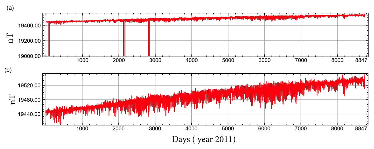
Figure 2
Typical example showing the data spikes in Z component of Alibag (ABG) observatory for 2011 and the corrected Z component values. (a) Unprocessed data set; (b) processed data set.
Table 2
Details of Data corrections and status of data for all stations used in this study. IAGA code is same as used in Table 1.
| IAGA CODE | BEFORE PROCESSING | SD (nT) | AFTER PROCESSING | SD (nT) | ||
|---|---|---|---|---|---|---|
| MIN (nT) | MAX (nT) | MIN (nT) | MAX (nT) | |||
| TIR | 1052 | 2499 | 289.6 | 1387 | 2438 | 289.6 |
| PND | 7500 | 8727 | 259.5 | 7708 | 8727 | 258.3 |
| VSK | 6501 | 18301 | 599.6 | 17080 | 18301 | 357.7 |
| ABG | 19000 | 20488 | 302.5 | 19412 | 20488 | 301 |
| NGP | 22000 | 23261 | 295.6 | 22202 | 23261 | 293.2 |
| RKT | 23001 | 24819 | 177.8 | 24190 | 24819 | 171.4 |
| SIL | 19001 | 29676 | 327.8 | 28625 | 29676 | 293 |
| ALH | 29000 | 32220 | 328.3 | 29367 | 30220 | 249 |
| SHL | 28001 | 30641 | 561.2 | 29261 | 30641 | 429.9 |
| JAI | 30500 | 31861 | 285.6 | 30797 | 31861 | 283.5 |
| GUL | 39500 | 40840 | 356.6 | 39648 | 40840 | 356.3 |
After putting these quality checks, 11 stations with 10 years of data were selected for the development of the gridded map. The methodology adopted are discussed in details below.
3. Experimental Methods
Spatio-temporal interpolation techniques for random fields is a commonly used practice to analyze how the field varies over time and space. It aims to use the existing dataset to estimate gaps and to find its spatial distribution ultimately (Willmott and Robeson, 1995; Anderson, 2002). Many statistical methods for interpolation emerge as promising solutions to estimate the signal values at the gap points. Few approaches that are applied often include inverse distance weighted and kriging procedures over many years (Gao and Revesz, 2006). The spatial interpolation techniques are mainly classified into three different categories: (i) geostatistical interpolation (non-deterministic), (ii) non-geostatistical interpolation (deterministic) and, (iii) combined methods (Li and Heep, 2014). Geostatistical interpolation techniques utilize the statistical properties of the measured data points, however; deterministic interpolation approach generates surfaces from measured values.
W. R. Tobler (1969) gave the first law of geography stating that the points which are close together in space are more likely to have similar values than points those are at a far distance. Similarly, the interpolation methods also use the neighborhood points to calculate the value at a different location. Many parameters like rainfall, chemical concentration, magnetic field, and noise pollution are predicted earlier using these methods (Haibin Li et al., 2024; Kit Fai Fung et al., 2022; Metahni et al., 2019; Taghizadeh-Mehrjardi et al., 2014). Presently, many spatiotemporal methods (e.g., Radial Basis Function, Polynomial Regression, Modified Shepard’s Method and Minimum Curvature methods) are used to estimate values at unsampled locations of the region. However, it is imperative to identify the inherent limitations associated with these different gridding methods (Bono et al., 2005; Yang et al., 2004; Eischeid et al., 2000; Metahni et al., 2019). For this study, different interpolation methods were utilized and compared with their ability to obtain the close to actual measurements giving low error. Also, as the magnetic data are received every second by the sensor in our case, the computational efficiency should also be very high. In the next section, we have explained different types of interpolation methods.
3.1 Methods for gridding
The method of spatial gridding involves collecting data z in a given location (x,y) (in the magnetic field is collected over different locations (longitude, latitude)) that is either irregularly or regularly spaced followed by interpolation or extrapolation of data to create a regularly spaced grid of z values at each grid node.
A grid node is the point where a row and a column intersect. Rows and column contain grid nodes with the same y and x coordinate respectively. Different methods use different mathematical algorithms to compute the weights during grid node interpolation, providing different representation of the data. The gridded data are used to generate contour maps in Surfer, which is a 3D modelling tool extensively used in contour mapping, surface mapping, or bathymetry modelling. Sometimes, the contour lines might be positioned differently relative to the original data as the locations of the contour lines are determined solely using the interpolated grid node values rather than the original data.
3.1.1. Kriging method (KRG)
When the problem of gridding of data arises, the most frequently used method is Kriging, which is considered very flexible and accurate. It describes spatial variation in terms of variograms and minimizes the error of predicted values estimated by its spatial distribution. The basic assumption of this methodology is that the distance between two sample points reveals a spatial correlation that can be used to explain spatial variation. Therefore, by taking into account the distance between neighboring observations a locally weighted average is used to estimate values at new points. Also, by giving the less weightage to clustered data, it can also compensate the clustered data. Each data point in Kringing is weighted by its distance from the grid node. In that case, the points that are far from the node will have less weight in the node estimation. Additionally, grid values can be extrapolated outside of the z value range of the data. The disadvantage of this method is that it is more time costlier than the other methods. This method has the capability of giving unbiased predictions with minimum variance and taking account of spatial correlation and statistical relationships between measured points (Krige, 1966).
3.1.2. Nearest Neighbour method (NAN)
Nearest Neighbour method (NAN) is undoubtedly the simplest interpolation one can consider, as it is not mathematically intense. It finds the closest subset of input samples to a query point and applies weights to them based on proportionate areas (Sibson, 1981). The z value of each grid node when using Nearest Neighbor is just the z value of the original data point that is closest to that grid node. In condition, where more than one point tie as the nearest neighbor, the tied data points are sorted first on x, then y, and then z values. It considers the smallest x value as the nearest neighbor. It is applied mainly with regularly spaced data points. This method also called exact interpolator, as it does not extrapolate beyond the z range of the data. In case of the data gaps, this method is best fitted. However, the algorithm’s sensitivity to the distance metric selection is a significant problem that can have a big impact on the model’s performance. In case of larger datasets, as the dimensionality enhanced the search for the nearest neighbors, it becomes time-consuming.
3.1.3. Natural Neighbour method (NEN)
The Natural Neighbor method is a more sophisticated technique that uses a weighted average of the values of neighboring points. The weights calculation are based on the proportion of the intersecting area of polygons of the known points. Compare to Nearest Neighbor, it provides smoother results as it tends to produce more continuous surfaces having gradual transitions. The disadvantage associated with the Natural Neighbor is the edge effects, which results where the interpolated values near the boundary may be less reliable due to the spars data coverage. It does not extrapolate contours beyond the convex hull of the data locations i.e., the outline of the Thiessen polygons (Yang et al., 2004).
3.1.4. Inverse Distance Weighting (IDW)
Inverse Distance Weighting (IDW) uses specific search distance, closest points, power setting, and barriers points to fill the gap between the data sets. This method calculates the weighted mean of nearby observations to find out the value z at location x. The weighting parameter is a function of the distance between the point of interest and the sampling points (Sun et al., 2009). To manage the impact of known values, it utilizes an additional variable in IDW called “power.” Nearby values will have more impact at higher powers. Although it is a fast method, it has the tendency to generate “bull’s-eye” patterns around the data points having of large number of contours. Also, it does not extrapolate values beyond the range of data.
3.1.5. Radial Basis method (RBF)
Like the Kriging method, the radial basis function (RBFs) method is flexible, giving accurate to interpolate multi-dimensional data. The real-value function derived in this method depends on the distance from the origin. Compared to the inverse distance weighting, RBFs creates even and less fluctuating values and handles larger datasets. The Radial Basis Function method takes the user-specified function and fits it through the data values. It uses a shaping factor R2, which provides a map with smooth contours and round mountain tops. The other important parameter is anisotropy ratio, which describes the relative weight of the points during interpolation. This ratio is achieved by dividing the maximum range to its minimum given range. The disadvantage of this method comes when it has large variation in surface values within short distances. Compared to the IDW, RBF is capable to predict values above the maximum and below the minimum measured values, however, IDW will never predict values above and below the extreme measured value (Johnston et al., 2001).
3.1.6. Polynomial Regression (POR)
According to the sample data, Polynomial Regression (POR) fits a mathematical surface, which is used to reflect the change of spatial distribution (Michael et al., 2016). This method is used for trend analysis regarding underlying large-scale trends and patterns. For any volume of data, polynomial regression is incredibly quick, but the resulting grid may lose local information in the data. By this technique, grid values can be extrapolated beyond the z range of the data. The Gridding method along with Kriging can eliminate the trend from their data or create 1st, 2nd, or 3rd order residual maps. In this combined approach, we first apply gridding using Kriging, and then use Polynomial Regression to identify the trend. Then, we subtract the Polynomial Regression grid from the Kriging grid to generate map of the resulting grid.
3.1.7. Triangulation with Linear Interpolation (TLP)
The Triangulation with Linear Interpolation method uses the optimal Delaunay triangulation when the data is evenly distributed entirely on grid area. The gridding method creates triangles by drawing lines between original data points considering no intersection of triangle by other triangles. This method is an exact interpolator but does not extrapolate data that is outside the data limits. The three initial data points that create a triangle determine its tilt and elevation, and each triangle defines a plane over the grid nodes that are within it (Yang et al., 2004). The triangular surface defines every grid node inside a particular triangle. The original data are rigorously used since they are utilized to define the triangles. The best results from triangulation with linear interpolation occur when the data are dispersed uniformly over the grid. Different triangular facets appear on the map when data sets with sparse areas are used.
3.1.8. Modified Shepard’s Method (MSM)
The Modified Shepard’s Method (MSM) uses modification of inverse distance weighted least squares method which can extrapolate values beyond the data’s z range. As it uses least squares, it does not tend to generate “bull’s eye” patterns as it reduces the expressive outliers that cause “bull-eyeing” effects. Modified Shepard’s Method can be either an exact or a smoothing interpolator. The Surfer algorithm implements a modified quadratic Shepard method of Franke and Nielson (1980), with full sector search as described in Renka (1988). By refining the iterative process, this method may reduce numerical errors, improving the precision of the solution. A disadvantage associated with this Method might is that it may not effectively handle outliers or anomalous data points. As the method is related to distance-based weighting, outliers can extremely affect the outcomes if they are included in the dataset.
3.1.9. Minimum Curvature Method (MNC)
This method is very quick and widely used in the earth sciences. It has the advantage to extrapolate values beyond data range. However, it can also create serious artifacts in case of data gaps. The interpolated surface created by Minimum Curvature resembles a thin, linearly flexible plate that passes through each data value with minimal curvature. In this method, two adjacent survey points are assumed to lie on a circular arc located in a plane. The orientation is defined by known inclination and direction angles at the ends of the arc (Bourgoyne et al., 1991). It fits the minimum curvature surface (i.e., the smoothest possible surface that matches the specified data values). It is best used when data is large and randomly distributed. This method is not an exact interpolator. These methods can be useful in some geophysical applications for simplifying data and models. However, they can also have significant disadvantages, particularly when dealing with complex geological environments or when high-resolution detail is required.
3.1.10. Moving Average (MOA)
This method is fast mostly applied very large data sets (e.g., >1,000 observations). It is designed in such a way that it can extracts information about intermediate-scale trends and variations from large and noisy data. This grid method provides a useful alternative to nearest neighbor for generating grids from large, evenly distributed data sets. This method has fast computation for larger number of datasets. In most GIS software (e.g., Surfer 8.0), the moving average method is implemented so as to assign values to points by averaging the data inside a user defined search area (Maleika, 2015).
3.1.11. Local Polynomial Method (LCP)
The Local Polynomial method is utilized especially for fitting polynomials to local subsets of data points in order to investigate the underlying structure preserved in a dataset. This method can model complex and non-linear relationships effectively. It adjusts the polynomial degree and bandwidth so it can adjust to multiple types of data patterns. The edge effect and computational complexity are some disadvantages associated with this method. LCP is capable of producing surfaces that may capture the short-range variation (Wang et al., 2014). The advantages and disadvantages of each of these methods are included in Table S2 of supporting information.
3.2 Experimental results and evaluation
In this study, using the data from the network of IIG observatories, we tested the different gridding methods to compute the earth magnetic field at the grid nodes. Many of these observatories are operating since 1972. The spatial interpolation uses the data sets from January 1st, 2011 to December 31st, 2020, as input to create the gridded Z field when maximum observatory data is available. At each station, data is sampled at every one minute. The spatial grid can create the gridded magnetic map at hourly resolution. An example of the gridded map using different methods for the year 2020 is shown in Figure 3. The yearly average magnetic field for 2020 is considered to obtain the spatial grid. Figure 3 shows the magnetic field variation over Indian region using IIG network through spatial interpolation as discussed in the previous section. It is seen that the MNC, MSM, NEN, TLC RBF, POR and KRG show clear spatial continuity. Interpolation using IDW, NAN, MOA shows a discontinuity around the nodal points. LCP shows edge effect. The gridding values are quantified and testified against the observations for reliability as discussed subsequently.
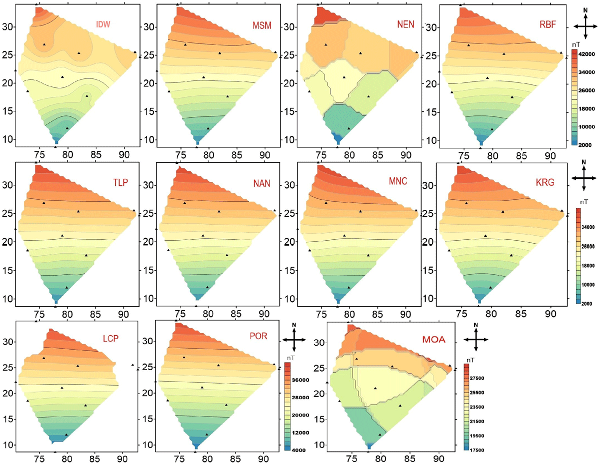
Figure 3
Results of different spatial interpolation method to get the magnetic field variation for Z component, over Indian region using IIG network for the year 2020.
We computed different statistical parameters for all the results obtained from interpolation methods applied to Z component magnetic field, averaged over the year 2020 (Table 3). The maximum (Max), minimum (Min), mean, and standard deviation (SD) are fundamental to analyze, as they provide essential information related to distribution and variability of a dataset. From the Table 3, we can see that each methods have the obvious margin (Min and Max values), except LCP, NAN, MOA, and POR. If we consider standard error aspect, MOA has smallest standard deviation. However, the minimum value achieved is very much deviated from those achieved by other methods and different from the actual values (at observatory sites). As the LCP, NAN, MOA, and POR have most of error in extreme and standard deviation (Table 3), we can consider KRG, MSM, RGF, and TLP for the given dataset.
Table 3
Statistical parameters for all the interpolation methods applied to magnetic field daily averaged data for the year 2020 (Z component).
| S.NO | INTERPOLATION METHOD | MIN (nT) | MAX (nT) | MEAN (nT) | S.D (nT) |
|---|---|---|---|---|---|
| 1 | Inverse distance to Power (INV) | 2375.374 | 40240.05 | 23981.01 | 6207.401 |
| 2 | Kriging (KRG) | 2906.175 | 39828.85 | 24631.17 | 7823.3 |
| 3 | Local Polynomial (LCP) | 4751.477 | 38744.21 | 23890.17 | 7643.955 |
| 4 | Minimum Curvature (MNC) | 2494.816 | 39893.56 | 24764.51 | 7998.209 |
| 5 | Modified Shepard’s Method (MSM) | 2961.5 | 40127.42 | 24826.6 | 7954.926 |
| 6 | Moving Average (MOA) | 17901.8 | 28798.71 | 23474.56 | 2366.748 |
| 7 | Natural Neighbor (NAN) | 3849.987 | 39839.23 | 24603.49 | 7722.897 |
| 8 | Nearest Neighbor (NEN) | 2027.8 | 40458 | 24381.98 | 8224.504 |
| 9 | Polynomial Regression (POR) | 4202.033 | 41453.94 | 24562.46 | 8041.312 |
| 10 | Radial Basis Function (RBF) | 2641.434 | 40067.2 | 24721.98 | 7947.856 |
| 11 | Triangulation With Linear Interpolation (TLP) | 2886.523 | 39851.7 | 24603.15 | 7892.121 |
In order to choose a specific interpolation method, each station is removed one by one and estimate the interpolated magnetic field at remaining locations are estimated by applying all the 11 methods. The difference between observed and interpolated values at each station are included in Table 4 for January 1st, 2015. This date is only a typical example where all the stations were operational. The difference is of the order of 102 nT for KRG, NEN, RBF, POR, MSM, MNC, and MOA for absolute data. For the other methods (NAN, IDW, TLP, and LCP), the departures are extremely large, which shows that these methods are not applicable for larger station gaps. Removing the stations TIR and RKT result in a NAN estimation from all methods as the grid scales lie outside of the study area. The average of the differences is included in the last row of Table 4. It is seen that the average of difference is smallest for NEN, followed by MSM. NEN method is not suitable for the current study where the observation location is very far from each other. Consideration of interpolation techniques discussed in section 4.1 shows that LCP included edge effects (also evident from Figure 3), and MOA needs a large point of observation to provide a meaningful interpolation. The RBF method, similar to KRG cannot be applied when the field variations are large. Both H and Z field absolute values show a large range of magnetic field variation from the southern station TIR to the northern station GUL (approximately 30000 nT). Some methods like NAN and IDW rely heavily on the spatial arrangement of data points. If the data points are unevenly distributed or clustered, the interpolation may not accurately reflect the underlying trend in less populated regions. If the data points are unevenly spaced, LCP and TLP methods may struggle in areas with sparse data, resulting in less accurate estimates. The data sets used in this study uses the geomagnetic field data from stations that are not equidistant from one another. In addition, spatial gridding involves edge effects especially at the boundary of the spatial grid. This leads to unrealistic values of interpolated values in many techniques. This is the reason that we obtain extreme values of 1038 of interpolated values for few methods (Table 4).
Table 4
Difference between observed and interpolated values (nT) of Z component (1 day averaged data for Jan 1st, 2015) after removing one by one station.
| METHODS | KRG | NAN | NEN | IDW | RBF | POR | TLP | MSM | MNC | MOA | LCP |
|---|---|---|---|---|---|---|---|---|---|---|---|
| NAG | 1.36E+03 | 1.23E+03 | –167 | 9.13E+02 | 1.30E+03 | 1.60E+03 | 1.06E+03 | 8.95E+02 | 8.15E+02 | –1.29E+02 | 2.40E+02 |
| POND | 1.51E+03 | –4.25E+37 | 6.25E+03 | –1.70E+38 | 2.36E+03 | 6.98E+02 | –4.25E+37 | 2.21E+03 | 3.02E+03 | –1.23E+04 | –1.70E+38 |
| SHL | –1.71E+03 | –1.70E+38 | –895 | –2.42E+02 | –2.04E+03 | –1.99E+03 | –1.28E+38 | –3.58E+03 | –3.80E+03 | 3.04E+03 | –3.01E+03 |
| ALA | 1.16E+03 | 6.91E+02 | 4.81E+03 | –1.70E+38 | 1.62E+03 | 3.57E+02 | 4.15E+02 | 7.78E+02 | 1.04E+02 | 5.83E+03 | 2.15E+02 |
| AIL | 9.80E+02 | –8.50E+37 | –4577 | 1.93E+03 | 1.11E+03 | 1.93E+03 | –4.25E+37 | –2.51E+02 | –2.51E+02 | –1.86E+03 | 1.29E+03 |
| VSK | –2.40E+03 | –1.35E+03 | –6616 | –4.67E+03 | –2.69E+03 | –1.13E+03 | –1.39E+03 | –1.74E+03 | –4.03E+02 | –5.59E+03 | –9.62E+02 |
| JAI | 3.77E+02 | –1.70E+38 | 0 | –1.70E+38 | 6.00E+01 | –1.82E+03 | –1.70E+38 | –1.54E+02 | –5.20E+02 | 1.25E+04 | –3.72E+01 |
| SIL | 2.62E+03 | –1.70E+38 | 895 | 1.52E+03 | 3.13E+03 | 3.13E+03 | –1.70E+38 | 4.06E+03 | 3.42E+03 | 4.87E+03 | 3.45E+03 |
| GUL | 3.99E+02 | –5.67E+37 | 0 | 9.71E+02 | 2.13E+02 | 60.31 | –5.67E+37 | –2.81E+02 | –1.50E+02 | 5.76E+03 | –1.58E+02 |
| RKT | NaN | NaN | NaN | NaN | NaN | NaN | NaN | NaN | NaN | NaN | NaN |
| TIR | NaN | NaN | NaN | NaN | NaN | NaN | NaN | NaN | NaN | NaN | NaN |
| Average | 4.77E+02 | –7.71E+37 | –3.33E+01 | –5.67E+37 | 5.63E+02 | 3.15E+02 | –6.77E+37 | 2.15E+02 | 2.48E+02 | 1.35E+03 | –1.89E+37 |
Subsequently, we estimate the RMSE for January 1st, 2015, from all the methods and at all geomagnetic observatories. We estimate the average of RMSE obtained at all sites and for all method. It is seen that the RMSE is minimum for MSM method (Table 5). Hence, after comparison of range and standard deviation from Table 3 and difference of observed and interpolated values from all eleven stations (Table 4), we consider the MSM as a probable method for interpolation of geomagnetic field.
Table 5
RMSE For 1-day averaged data (Jan 1st, 2015) for 11 different methods at 11 observatories.
| OBS. | KRG | NAN | NEN | IDW | RBF | POR | TLP | MSM | MNC | MOA | LCP |
|---|---|---|---|---|---|---|---|---|---|---|---|
| TIR | 708.9 | 1.70E+38 | 0 | 732.1 | 1458.2 | 1331.3 | 1.70E+38 | 85.04 | 658.1 | 13635.2 | 75.5 |
| PND | 1842.3 | 8.51E+37 | 0 | 825.0 | 1640.9 | 1578.9 | 8.51E+37 | 2013.4 | 2423.9 | 10717.7 | 2102.8 |
| VSK | 565.9 | 632.8228 | 0 | 760.4 | 1543.2 | 962.9 | 690.9 | 284.5 | 519.6 | 5031.4 | 108.0 |
| ABG | 1356.6 | 1.20E+38 | 0 | 502.2 | 1547.4 | 2066.3 | 8.51E+37 | 1244.7 | 1300.6 | 1657.7 | 1397.7 |
| NGP | 1998.9 | 1894.744 | 0 | 656.3 | 1698.3 | 2074.9 | 1875.3 | 1824.8 | 1819.7 | 117.5 | 1935.8 |
| RKT | 1151.6 | 1.70E+38 | 0 | 214.3 | 1289.0 | 1511.4 | 1.70E+38 | 1084.3 | 1105.9 | 2919.2 | 1207.2 |
| SIL | 1392.2 | 1.70E+38 | 0 | 458.3 | 385.8 | 2619.7 | 1.70E+38 | 284.9 | 2636.7 | 3879.6 | 1274.2 |
| ALH | 1120.5 | 1106.886 | 0 | 993.7 | 1420.2 | 1394.2 | 1119.3 | 1670.2 | 1689.8 | 5340.6 | 1469.6 |
| SHL | 989.3 | 1.47E+38 | 447.5 | 406.2 | 736.8 | 1976.7 | 1.47E+38 | 612.1 | 3499.0 | 2523.5 | 793.2 |
| JAI | 1532.3 | 1462.13 | 0 | 867.2 | 1385.5 | 1637.3 | 1475.0 | 1743.4 | 1751.3 | 5693.8 | 1445.6 |
| GUL | 379.2 | 1.70E+38 | 0 | 617.4 | 870.5 | 1947.0 | 1.70E+38 | 426.9 | 739.3 | 11869.5 | 64.5 |
| Average RMSE over all stations | 1185.24 | 9.38E+37 | 447.5 | 639.37 | 1270.53 | 1736.42 | 9.07E+37 | 1025 | 1649.45 | 5762.34 | 1079.46 |
4. Development of MATLAB GUI and application
A user-friendly MATLAB GUI is created using MATLAB app compatible with version 2023b. The GUI can provide the gridded H and Z geomagnetic field components of India for every hour. The developed GUI has inbuilt averaging and gridding techniques (Details of the MATLAB GUI are included in the text file as supplementary, and can be executed on MaTLAB2023b version or higher). A total of 15 × 15 (total 225) grid points with a spatial separation of 250 km × 250 km is used to generate the GUI. The interactive GUI provides the user with RMSE error between the observatory value and interpolated values. User can choose the number of contour lines for the geomagnetic field data. The GUI snapshot is shown in Figure 4. Using this GUI, both total field and variation field can be visualized. An example of total field for the year 2011 (where three stations were not operational) and 2017 (where all observatories were operational) using the GUI is shown in Figure 5. As it is evident the horizontal magnetic field shows an increase near the geomagnetic equator with decreasing amplitude toward the northern latitude stations in India. At the equator, the H component shown an amplitude of approximately 40,000 nT and low latitude stations the H component has 37,000 nT. In the similar manner, contours of vertical component Z also show a decrease toward equator with values as low as 4000 nT near southern part of India and 31000 nT in the northern part of India (Figure 5). It should be noted that the Port Blair station data is not used while preparing the GUI. The year 2011 indicates the ascending phase of solar cycle, whereas 2017 indicates the descending phase of the solar cycle. These effects can be captured in the variation mode of GUI.
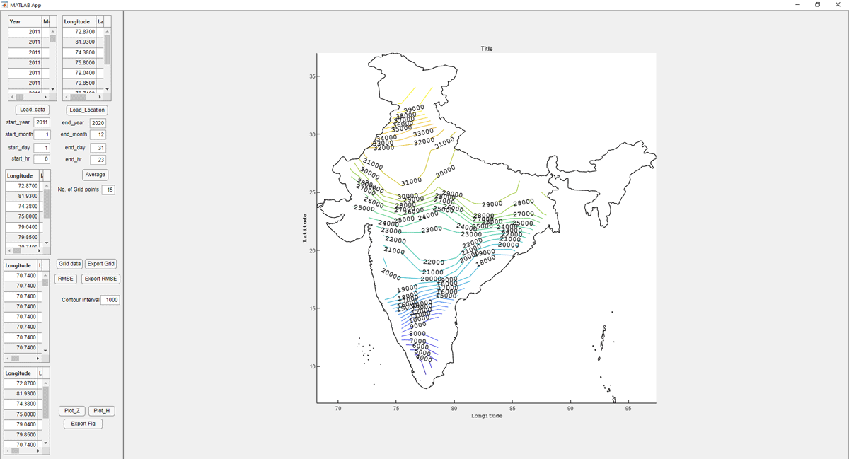
Figure 4
Snapshot of MATLAB based GUI for obtaining the interpolated contour for H and Z magnetic field components.
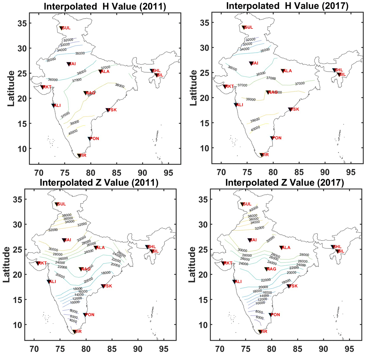
Figure 5
Gridded magnetic field components (a) H and (b) Z for the year 2011.
Using this GUI, the daily, monthly, and seasonal variabilities of geomagnetic field components can be generated. The monthly variation of interpolated Z field averaged over India is shown Figure 6a (dashed lines). The corresponding monthly average from observed magnetic field, averaged over India is also included in the same panel (solid lines). It is seen that the monthly average observed and interpolated values show as similar trend for most of the months. However, the interpolated fields overestimate the magnetic field by 1000 nT, which is equivalent to the RMSE error through MSM method. Panels (b) and (c) of Figure 6 indicate the observed values of Z field at TIR and ABG respectively for one minute sampling resolution. during 2011–2020. Panel (d) shows the variation of interpolated Z field at ABG in hourly resolution during 2011–2020.
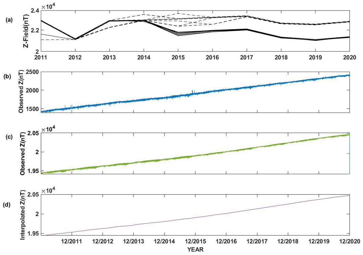
Figure 6
Variations of total H and interpolated and observed Z field components for the years 2011–2020, created using MATLAB GUI. Panels (a), indicate the monthly variation of interpolated (dashed lines) and observed (solid lines) Z values for entire India. Panels (b) and (c) indicate the observed values of Z field at TIR and ABG respectively in minute resolution during 2011–2020. Panel (f) shows the variation of interpolated Z field at ABG location during 2011–2020.
The observed Z field clearly indicates an increase of 100 nT per year at TIR and ABG (Panels (b) and (c)). The same trend is seen for all other observatories (not shown here). It is interesting to note that this trend is also reproduced by the interpolated Z field at ABG coordinates. This demonstrates the application of the developed GUI.
It should be noted that the MATLAB GUI results shown here are only considered the absolute values of the data sets and not the variation of the magnetic field. The error of estimation of the absolute magnetic field is 1000 nT from the interpolated result. Thus, the GUI can be used while addressing changes over decadal scales. In case of transient events, like geomagnetic storms where the magnetic field change is within 50–100 nT, the input magnetic field file should contain the variation data alone and not the absolute data as is illustrated for Figure 5. An example of the gridded magnetic map for short term transient event is shown in Figure S1 in the supporting information. To create the spatial grid for variation data, the input field is prepared using variation field data from all stations during 2011–2020. Figure S1 shows the changes in the H and Z gridded magnetic map on March 10th, 2015 (International Quiet day) and on March 17th, 2015 (St. Patrick’s Day). It is interesting to note that there is a clear reduction in the H field amplitude from quiet day on March 10th, 2015 to disturbed day on March 17th, 2015 by 100 nT near the equatorial latitude, which was observed globally from other longitudes as well (Bulusu et al., 2018). Thus, by using the appropriate input file, both absolute field and variation field gridded map can be created using this MATLAB GUI.
5. Discussion
Spatial gridding is a traditional method to understand the gradients in many physical parameters like magnetic anomalies, rain fall, etc. These studies involve the usage of different methods discussed in section 4. For example, Kit Fai Fung et al. (2022) applied interpolation methods like IDW and Ordinary Kriging (OK) for mapping the rainfall distribution in peninsular region of Malaysia. Haibin Li et al. (2024) proposed an improved Kriging interpolation method to enhance the spatial resolution of magnetic anomaly features. In the current study, we are using the Modified Shepard method to obtain the gridded geomagnetic field map of India using 10 years of magnetic field data.
The gridding can be performed on both the absolute and variation magnetic field data. The quality control of data sets is a prerequisite and as well as crucial to preparation of gridded data set. After optimizing the data continuity, the gridded magnetic field is created for both absolute and variation field of H and Z components. The minimum error of gridded data with respect to observed values is approximately 1000 nT in case of absolute values and 50 nT in case of variation field. It should be noted that the gridded data set is prepared with interpolation technique, hence the estimated values would be only an approximate value of the observed field variations at the grid nodes. The accuracy of the gridded data is tested using observatory data. The gridded data set can be used to both quickly look charts of magnetic field variation and also to identify long-term geomagnetic field anomalies.
Each contour in the map connects the magnetic field of similar values and the density of contour lines indicate the slope of the gradient in the field values. For example, the contours of H component indicate a larger value close to the equator that decreases in its value toward lower latitudes (Figure 5). In addition, the density of contour lines is sparse and distributed at larger distances, indicating the gradient in the field is gradual, especially in the central part of India. In case of Z field mapping, a minimum value of approximately 4000 nT is observed near the equator, increasing to 38000 nT at lower latitudes. Further, the density of contour lines is closely spaced with varied intensities indicating a steeper gradient in Z field absolute values.
The variation field of H and Z mapping indicates interesting clustering and steep variation of H and Z field (Figure S1). The gridded map has an additional advantage that the method can be used in the absence of one or more stations as illustrated in Table 4.
6. Conclusions
This is the first gridded regional magnetic field map of India that represents the absolute and variations of the magnetic field in Indian regions. In this paper, we present a geomagnetic field data grid over Indian region (8° to 32° N and 70° to 92° E), generated using the geomagnetic field data from the 11 geomagnetic observatories with a resolution of 250 × 250 km during the years 2011–2020. Currently, 225 grid points are used in the GUI which can be modified based on availability and separation between observation points.
The contour plot can be generated to account contributions from both ionospheric and internal magnetic field variations separately. The geomagnetic field variation of H components shows an increase at equator of 40000 nT and decreases toward the northern low latitudes. The Z shows a minimum at the equator and incases toward the northern low latitudes. Further, the steep gradients in the H and Z field can be accessed by density of contour lines. The gridded map is currently presented for the recent years of 2011–2020 using data from the available 11 geomagnetic observatories operated by Indian Institute of Geomagnetism. The developed MATLAB GUI is applicable to both absolute and variation of magnetic field. The GUI may be used to generate the magnetic field variations from older times when only a few stations were spatially and temporally recording the magnetic field variations in India.
Data Accessibility Statements
Data used in the study will be made available on request by emailing at iig.director@iigm.res.in.
Additional File
The additional file for this article can be found as follows:
Supplementary File
Appendix MATLAB GUI for Gridded map of India. DOI: https://doi.org/10.5334/dsj-2025-010.s1
Acknowledgements
Figure 3 is plotted using inbuilt program of SURFER software. The research is carried out as an initiative from Director’s Research Group.
Competing Interests
The authors have no competing interests to declare.