
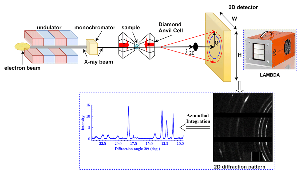
Figure 1
Schematic diagram of the High Energy Density (HED) experiment setup.
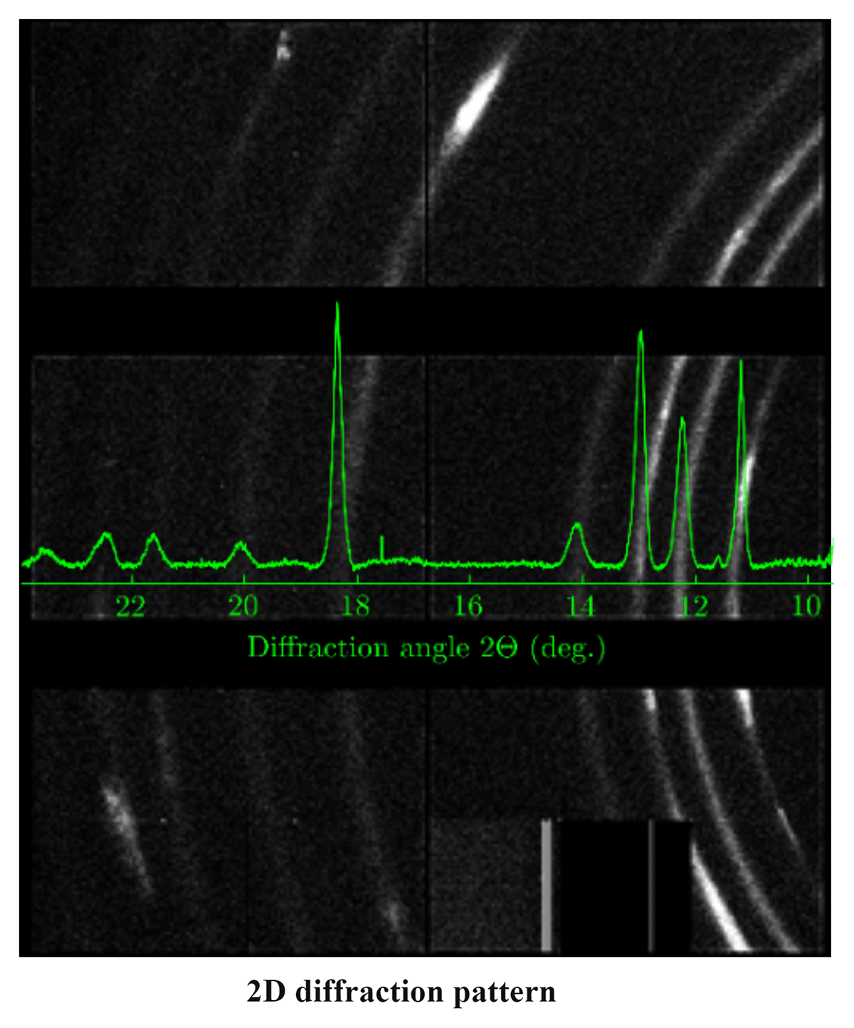
Figure 2
Raw X-ray diffraction image from a (Mg0.2Fe0.8)O magnesiowüstite sample collected with the LAMBDA GaAs 2M detector. This figure was measured at PETRA III beamline P02.2 using a 25.6 keV beam. The 2D raw diffraction image shows the starting condition at 1 GPa and with fcc/B1 (Mg0.2Fe0.8)O sample. After azimuthal integration, the corresponding 1D spectrum is shown in green on top of it.
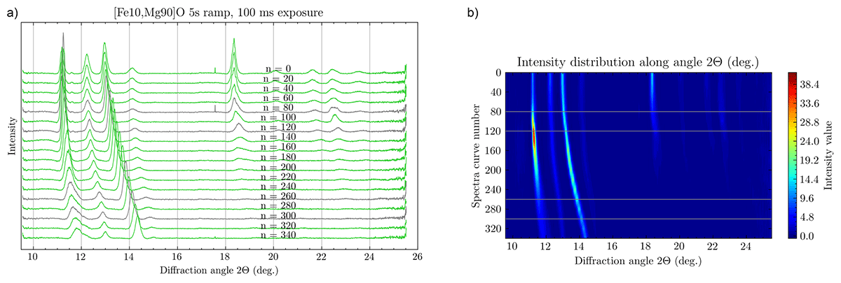
Figure 3
(a) Spectral data (one for every 20 diffiractograms) collected during the experiment after baseline subtraction, and (b) Contour maps of Intensity distribution of each diffractogram along 2θ axis. Note that 4 spectra are grayed out which were randomly picked as the basis for the ML training set for representing the two experimental states (before and after phase transition).
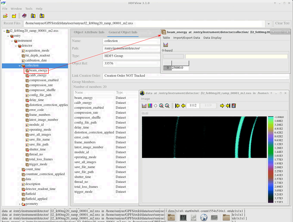
Figure 4
An hdf5 experimental raw data file is displayed in HDFview software.
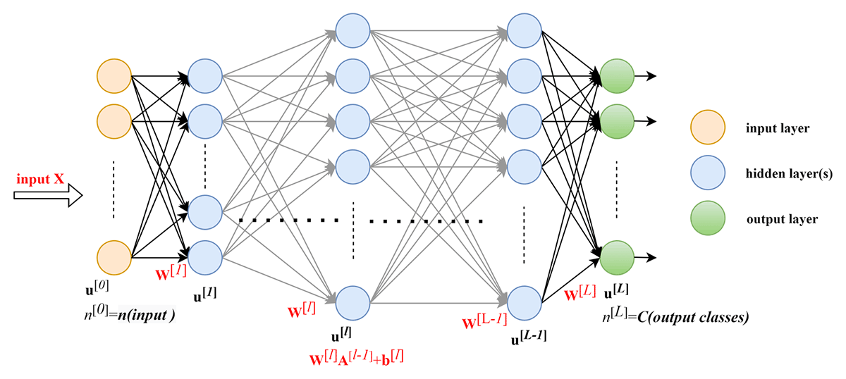
Figure 5
A multilayer deep fully connected network.
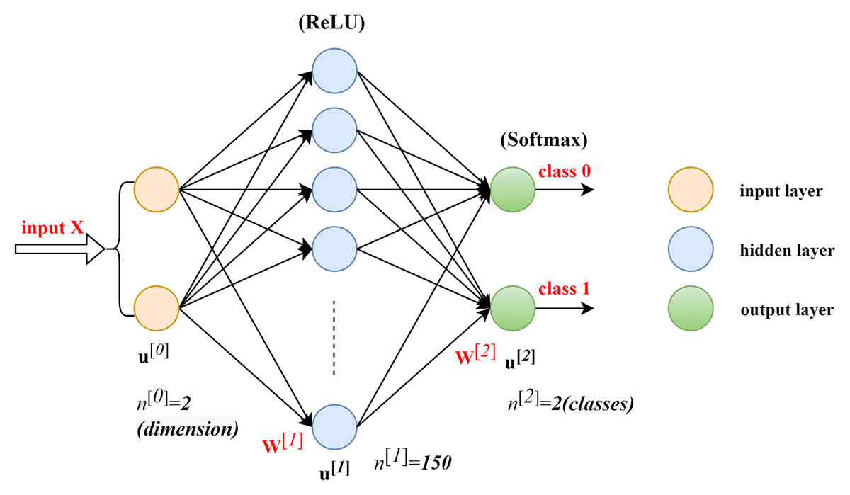
Figure 6
Two-layered neural network structure used for spectra classification.
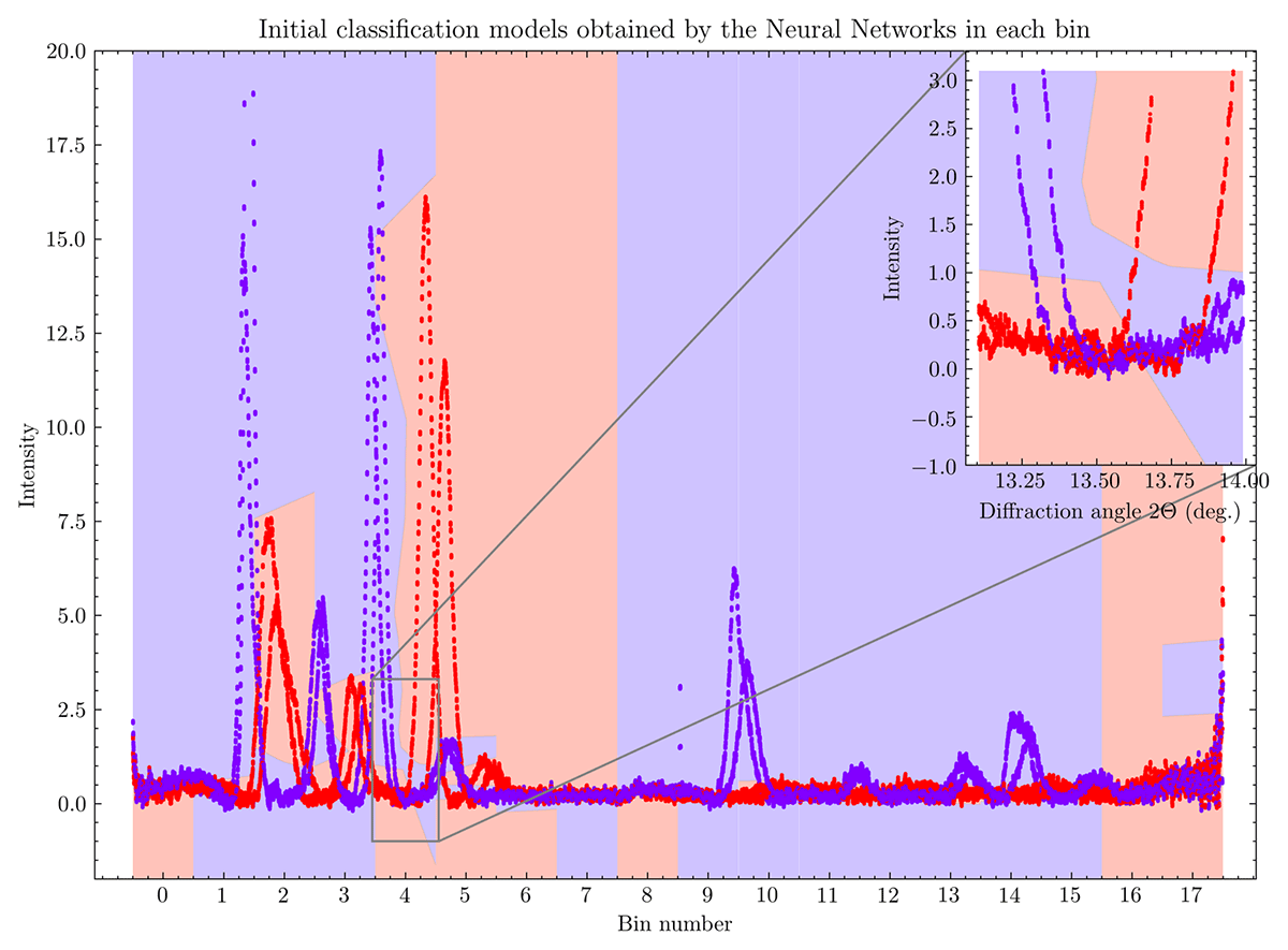
Figure 7
The initial classification model for each bin obtained by the respective trained two-layered network models.
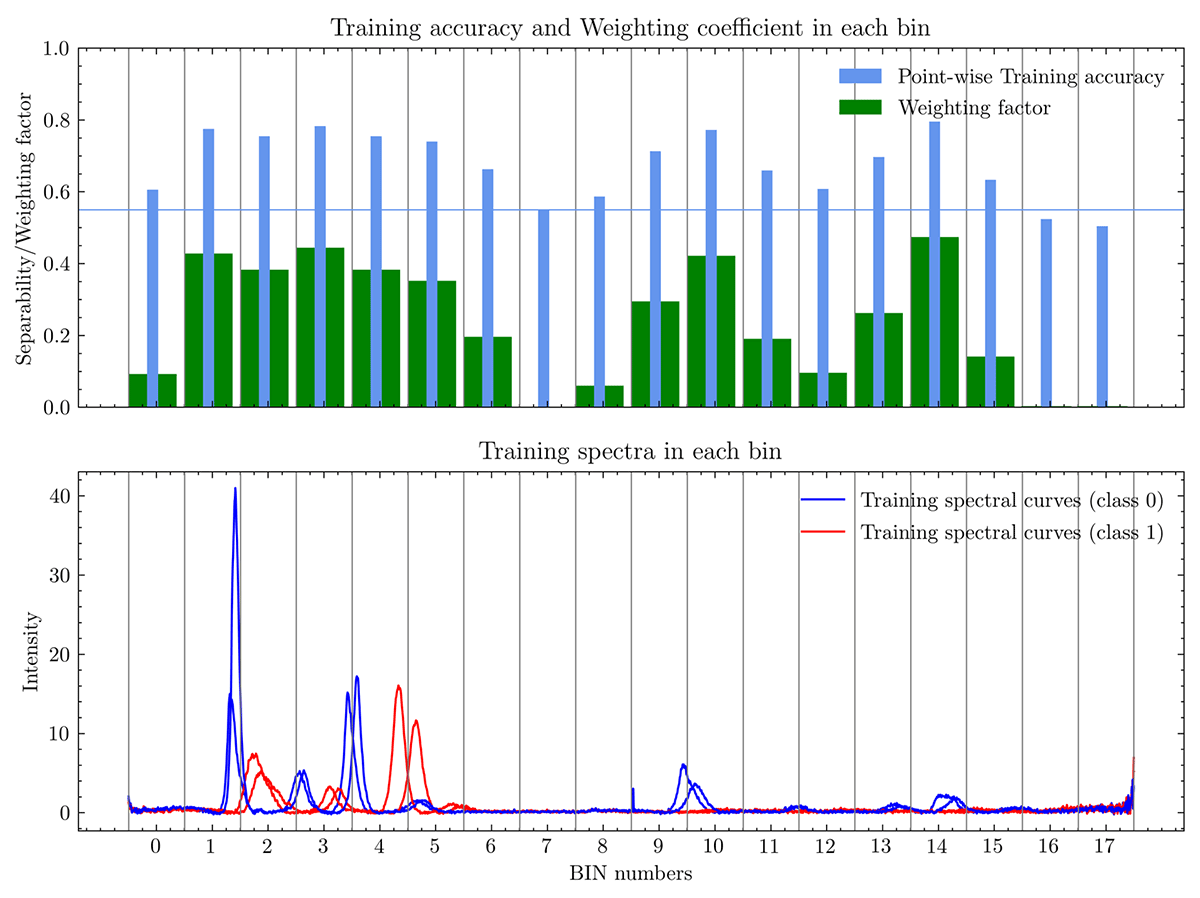
Figure 8
The distribution of point-wise training accuracy (separability), and the believability weighting factor for each bin.
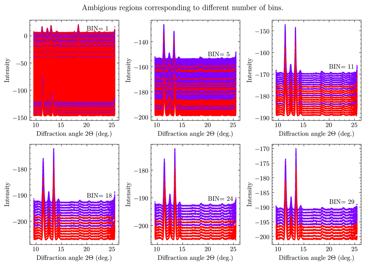
Figure 9
Final classification result of test spectral curves near the boundary (using 1, 5, 11, 18, 24, 29 bins). The spectrum is pulled evenly by moving the Intensity baseline for better display.
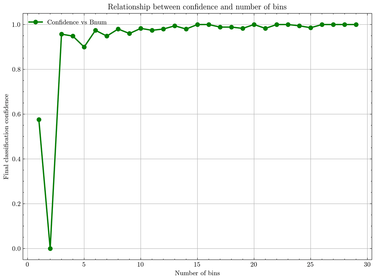
Figure 10
Relationship between final classification accuracy and number of bins.